Satellite Environmental MonitoringPemantauan Lingkungan Berbasis Satelit


pip install earthchange
A hands-on tutorial. Map deforestation, mining, urbanisation, floods, burns and surface-water change anywhere on Earth from free satellite data — then export georeferenced GeoTIFFs and print-ready maps. All in Python, powered by Google Earth Engine and Microsoft Planetary Computer.
Tutorial praktis. Petakan deforestasi, tambang, urbanisasi, banjir, kebakaran, dan perubahan air permukaan di mana saja dari data satelit gratis — lalu ekspor GeoTIFF tergeoreferensi dan peta siap cetak. Semua dengan Python, ditenagai Google Earth Engine dan Microsoft Planetary Computer.
Why this existsMengapa perangkat lunak ini ada
Satellite data has been free for years. The ability to use it has not. The imagery is there — Sentinel, Landsat, MODIS, decades of it, downloadable by anyone. What stands between those images and an answer is a stack of things that take months to learn: cloud masking, projections, which index suits which question, what threshold deserves to be called "change", and how to turn a raster into a number someone can act on. Yet the people who most need the answer — a district forestry officer, an NGO researcher, a journalist on deadline, a lecturer preparing a class, a student with three months left — are often precisely the people without those months. So the question this package asks is a narrow one: can a single command do the whole thing?
Data satelit sudah gratis bertahun-tahun. Kemampuan memakainya belum. Citranya ada — Sentinel, Landsat, MODIS, berpuluh tahun, bisa diunduh siapa saja. Yang berdiri di antara citra itu dan sebuah jawaban adalah tumpukan hal yang perlu berbulan-bulan untuk dikuasai: penapisan awan, sistem proyeksi, indeks mana untuk pertanyaan mana, ambang berapa yang pantas disebut "berubah", dan bagaimana mengubah raster menjadi angka yang bisa ditindaklanjuti orang. Sementara mereka yang paling membutuhkan jawabannya — penyuluh kehutanan di kabupaten, peneliti lembaga swadaya, wartawan yang dikejar tenggat, dosen yang menyiapkan kuliah, mahasiswa yang tinggal punya tiga bulan — justru sering kali adalah orang-orang yang tidak punya bulan-bulan itu. Maka pertanyaan yang diajukan paket ini sempit saja: bisakah satu baris perintah mengerjakan seluruhnya?
A function you use again and againFungsi yang dipakai berulang-ulang
The answer this package gives is not a script you adapt. It is a ready-made analysis — the method, the thresholds, the masking and the output already decided — and the only things you change are where and when. Those two are the whole interface:
Jawaban yang diberikan paket ini bukan skrip yang harus Anda sesuaikan. Ia adalah analisis siap pakai — metode, ambang, penapisan, dan bentuk keluarannya sudah ditetapkan — dan yang Anda ubah hanyalah di mana dan kapan. Keduanya adalah seluruh antarmukanya:
# Ketapang, 2019
earthchange -s fire-danger --admin Ketapang --date 2019-09-30

# the same analysis, somewhere else, another year
earthchange -s fire-danger --admin "Kalimantan Tengah" --date 2026-08-01
Nothing was written between those two lines. No index chosen, no cloud mask configured, no projection set, no colour ramp designed. That is what "ready to use" has to mean if it is to be worth anything: copy, change two words, run — and out come a map you can put in front of a bupati, a GeoTIFF for the GIS staff, and a JSON of numbers for the report. A novice never opens a code editor.
Tidak ada satu baris pun yang ditulis di antara kedua perintah itu. Tidak memilih indeks, tidak menyetel penapis awan, tidak mengatur proyeksi, tidak merancang gradasi warna. Itulah yang harus berarti "siap pakai" agar ada gunanya: salin, ubah dua kata, jalankan — dan keluarlah peta yang bisa disodorkan kepada bupati, GeoTIFF untuk staf GIS, dan JSON angka untuk laporan. Pengguna pemula tidak pernah membuka editor kode.
This is deliberately not a toolbox. A general GIS platform hands you a thousand operations and asks which sequence answers your question; that is the right tool for someone who already knows the answer to that. This is for the far larger group who have the question but not the method — who need to know whether a district is drying, not which spectral index to subtract from which. Both kinds of software should exist. They are not substitutes.
Ini memang sengaja bukan kotak perkakas. Platform GIS umum menyodorkan seribu operasi lalu bertanya urutan mana yang menjawab pertanyaan Anda; itu perkakas yang tepat bagi orang yang sudah tahu jawabannya. Yang ini untuk kelompok yang jauh lebih besar — mereka yang punya pertanyaannya tetapi bukan metodenya, yang perlu tahu apakah sebuah kabupaten sedang mengering, bukan indeks spektral mana yang harus dikurangkan dari mana. Keduanya perlu ada. Keduanya bukan pengganti satu sama lain.
One honest wrinkle. "Just change the date" holds completely for a season that has ended. For anything recent it does not: the archives run between one day and three months behind, each by a different amount, so the newest date that works shifts daily and differs by scenario. The package will tell you which date to use rather than fail obscurely — but it is the one part of the copy-and-paste promise that needs a little care.
Satu catatan jujur. "Tinggal ganti tanggalnya" berlaku sepenuhnya untuk musim yang sudah berakhir. Untuk data terkini tidak: arsipnya tertinggal antara satu hari sampai tiga bulan, masing-masing berbeda, sehingga tanggal terbaru yang bisa dipakai bergeser tiap hari dan berbeda antar skenario. Paket ini akan memberi tahu tanggal mana yang bisa dipakai, bukan gagal tanpa penjelasan — tetapi inilah satu bagian dari janji salin-tempel yang perlu sedikit kehati-hatian.
ObjectivesTujuan
- One command, one question. No Earth Engine scripting, no threshold to choose, no projections to manage.
- Calibrated where it runs. Fire danger classes follow BMKG, not Canada. Day-length factors use the equatorial convention, because the standard tables were drawn up for 46°N. Drought Code leads over FWI, because peat fire is driven by deep drying. Air quality uses ISPU. Global tools are calibrated for everywhere, which means for nowhere in particular.
- Outputs you can actually use. A print-ready A4 map sheet, a GeoTIFF that opens straight in QGIS, statistics as JSON, and text in Indonesian and English.
- Your own data, not only global layers. Rice-field boundaries, forest designation, an authoritative peat map — crossed with public satellite data. That is the difference between "West Kalimantan is dry" and "87% of this nature reserve is dry".
- Honest about its limits. Every output states what it cannot tell you. A tool that hides its limits misleads precisely when it is trusted most.
- Free, open and citable. MIT licence, Zenodo DOI.
- Satu perintah untuk satu pertanyaan. Tidak perlu menulis skrip Earth Engine, tidak perlu memilih ambang, tidak perlu mengurus proyeksi.
- Dikalibrasi di tempat ia dipakai. Ambang bahaya kebakaran mengikuti BMKG, bukan Kanada. Faktor panjang hari memakai konvensi ekuatorial, karena tabel bakunya disusun untuk 46°LU. Drought Code dipimpinkan di atas FWI, karena kebakaran gambut didorong pengeringan lapisan dalam. Kualitas udara memakai ISPU. Perkakas global dikalibrasi untuk seluruh dunia — yang berarti tidak untuk tempat mana pun secara khusus.
- Keluaran yang benar-benar bisa dipakai. Lembar peta A4 siap cetak, GeoTIFF yang langsung terbuka di QGIS, statistik JSON, teks dwibahasa.
- Data Anda sendiri, bukan hanya data global. Lahan baku sawah, batas fungsi kawasan, peta gambut resmi — disilangkan dengan data satelit publik. Inilah yang membedakan "Kalimantan Barat kering" dari "87% cagar alam ini kering".
- Jujur tentang batasnya. Tiap keluaran menyebutkan apa yang tidak bisa ia katakan. Perangkat yang menyembunyikan batasnya akan menyesatkan tepat pada saat ia paling dipercaya.
- Gratis, terbuka, dapat disitasi. Lisensi MIT, DOI Zenodo.
The hopeHarapan
The measure of this package is not downloads. It is whether an analysis that would never have happened, happens — because the person who needed to answer the question no longer had to become a remote sensing specialist first. A lecturer teaches with it. A student finishes a thesis with it. An organisation publishes a number that others can check. A district official sees which areas are drying, before they burn. And a further hope: that people take this approach to their own places. BMKG's thresholds suit Indonesia and nowhere else, but the idea that a tool should be calibrated for where it is used — and should say what it does not know — travels anywhere.
Ukuran keberhasilan paket ini bukan jumlah unduhan. Ukurannya adalah apakah ada analisis yang tadinya tidak akan pernah terjadi, akhirnya terjadi — karena orang yang perlu menjawab pertanyaannya tidak lagi harus lebih dulu menjadi ahli penginderaan jauh. Seorang dosen memakainya untuk mengajar. Seorang mahasiswa menyelesaikan skripsinya dengannya. Sebuah lembaga menerbitkan angka yang bisa diperiksa orang lain. Seorang pejabat kabupaten melihat kawasan mana yang sedang mengering, sebelum ia terbakar. Dan harapan yang lebih jauh: bahwa orang mengambil pendekatan ini untuk tempat mereka sendiri. Ambang BMKG hanya cocok untuk Indonesia, tetapi gagasan bahwa sebuah perkakas harus dikalibrasi untuk tempat ia dipakai — dan harus mengatakan apa yang tidak diketahuinya — berlaku di mana saja.
1 · What you'll buildYang akan Anda buat
By the end you'll run a single command like this…
Di akhir tutorial, Anda menjalankan satu perintah seperti ini…
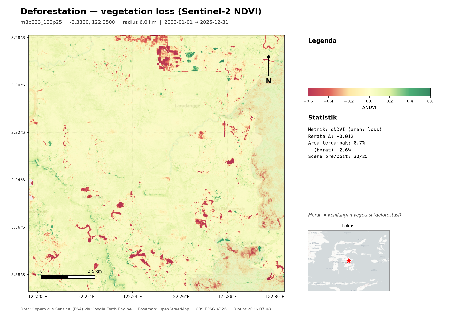
earthchange -s deforestation --lat -3.333 --lon 122.25 --radius 6 --map…and get three things for your chosen area:
…dan mendapat tiga berkas untuk area pilihan Anda:
- a quick-look PNG of the change,
- a full-resolution, georeferenced GeoTIFF you can open in QGIS/ArcGIS, and
- a value-added map (A4 PDF + PNG) with legend, scale bar, statistics and a location inset.
Cloud and shadow are the main source of false positives, and the direction is not random: shadow depresses NIR more than SWIR, so it lowers both NDVI and NBR — it mimics vegetation loss and burn, never gain. Per-pixel cloud masking plus a median over many scenes absorbs most of that, but a median over one clear look simply reproduces whatever the mask missed. Change is therefore only reported where both windows have at least --min-obs cloud-free looks at that pixel (default 2); the excluded share is printed and recorded in stats.clear_observations. Raise it to 3–4 in persistently cloudy areas, --min-obs 1 to disable. What this does not fix: a pixel with many looks that are all shadowed the same way — seasonal terrain shadow, for instance — passes the count test and still biases the result.
Awan dan bayangan adalah sumber utama positif palsu, dan arahnya tidak acak: bayangan menurunkan NIR lebih besar daripada SWIR, sehingga menurunkan NDVI maupun NBR — ia menyerupai kehilangan vegetasi dan kebakaran, tidak pernah pertambahan. Mask awan per piksel plus median banyak scene meredam sebagian besar hal itu, tetapi median dari satu pengamatan bersih hanya mengulang apa pun yang lolos dari mask. Karena itu perubahan hanya dilaporkan bila kedua jendela punya minimal --min-obs pengamatan bebas awan pada piksel tersebut (bawaan 2); porsi yang dikecualikan dicetak dan dicatat di stats.clear_observations. Naikkan ke 3–4 di wilayah yang terus berawan, --min-obs 1 untuk menonaktifkan. Yang belum teratasi: piksel dengan banyak pengamatan yang semuanya terbayang dengan cara sama — misalnya bayangan topografi musiman — lolos uji jumlah dan tetap membiaskan hasil.
Optical scenarios also write a SWIR false-colour quick-look of each source composite — the pre and post imagery the change was measured between — and record every scene that went into them (id, date, cloud %) under images_used in stats.json. A count alone can be neither checked nor reproduced; the ids can. Use --no-preview to skip both.
- PNG pratinjau perubahan,
- GeoTIFF resolusi penuh tergeoreferensi yang bisa dibuka di QGIS/ArcGIS, dan
- peta value-added (A4 PDF + PNG) dengan legenda, skala, statistik, dan inset lokasi.
Skenario optik juga menuliskan pratinjau warna semu SWIR untuk tiap komposit sumber — citra pra dan pasca yang menjadi dasar pengukuran perubahan — serta mencatat setiap scene yang menyusunnya (id, tanggal, % awan) pada images_used di stats.json. Jumlah scene saja tidak bisa diperiksa maupun direproduksi; id-nya bisa. Pakai --no-preview untuk melewati keduanya.
You pick a scenario (what kind of change) and a location (a coordinate). The tool selects the right remote-sensing method automatically. No prior GIS coding required.
Anda memilih skenario (jenis perubahan) dan lokasi (koordinat). Alat memilih metode penginderaan jauh yang tepat secara otomatis. Tanpa perlu pengalaman pemrograman GIS.
2 · How it works (the science)Cara kerjanya (sainsnya)
“Change detection” compares the landscape at two (or more) points in time and highlights what changed. Different phenomena leave different spectral or radar fingerprints, so each scenario uses a purpose-built index or method:
“Deteksi perubahan” membandingkan bentang lahan pada dua (atau lebih) titik waktu dan menonjolkan apa yang berubah. Fenomena berbeda meninggalkan sidik jari spektral atau radar yang berbeda, sehingga tiap skenario memakai indeks atau metode khusus:
| ScenarioSkenario | Method & formulaMetode & rumus | Sensor | BasisDasar |
|---|---|---|---|
| deforestation | ΔNDVI < 0. NDVI = (NIR−Red)/(NIR+Red) = (B8−B4)/(B8+B4). Vegetation loss lowers NDVI.Kehilangan vegetasi menurunkan NDVI. | Sentinel-2 | NDVI (Rouse 1973; Tucker 1979) |
| urbanization | ΔNDBI > 0. NDBI = (SWIR−NIR)/(SWIR+NIR) = (B11−B8)/(B11+B8). Built-up reflects more SWIR.Permukaan terbangun memantulkan lebih banyak SWIR. | Sentinel-2 | Zha et al. 2003 |
| burn | dNBR. NBR = (NIR−SWIR2)/(NIR+SWIR2) = (B8−B12)/(B8+B12). Burns lower NBR.Kebakaran menurunkan NBR. | Sentinel-2 | Key & Benson 2006 |
| water | ΔNDWI. NDWI = (Green−NIR)/(Green+NIR) = (B3−B8)/(B3+B8). | Sentinel-2 | McFeeters 1996 |
| flood | SAR water: smooth water gives low VV backscatter. Uses one pre scene and one post scene from the same relative orbit (the latest pass in each window) — the standard S1 method, not a window average. Flood = water in the post scene but not the pre scene. Permanent water & the ocean are masked (ESA WorldCover). The two acquisition dates are reported in the stats and on the map.Air SAR: air halus memberi backscatter VV rendah. Memakai satu citra pra dan satu citra pasca dari orbit relatif yang sama (lintasan terbaru di tiap jendela) — metode S1 baku, bukan rata-rata jendela. Banjir = air pada citra pasca tetapi tidak pada citra pra. Air permanen & laut di-mask (ESA WorldCover). Kedua tanggal akuisisi ditampilkan di statistik dan peta. | Sentinel-1 | UN-SPIDER |
| disturbance | Impact mapping where water detection fails — forested hills, flash floods, landslides. Vegetation/structure removed → VH backscatter drops. Uses one pre + one post scene (same relative orbit); flags where VH fell >3 dB (severe >6 dB). SRTM slope attributes steep drops as landslide-like vs flat drops as sediment/inundation-like. Use this when flood shows nothing over terrain.Pemetaan dampak saat deteksi air gagal — perbukitan berhutan, banjir bandang, longsor. Vegetasi/struktur hilang → backscatter VH turun. Memakai satu citra pra + satu pasca (orbit relatif sama); menandai VH turun >3 dB (berat >6 dB). Lereng SRTM mengklasifikasi penurunan di lereng curam sebagai mirip longsor vs di dataran sebagai mirip endapan/genangan. Pakai ini saat flood tak menampilkan apa pun di medan bergunung. |
Sentinel-1 | SAR VH change + slopePerubahan VH SAR + lereng |
| smoke-track | Which way the wind carried the smoke — indicative forward trajectories. smoke-exposure answers who breathed it; this answers where it went. Air parcels are seeded on the day's hottest FIRMS detections and carried forward on the hourly ERA5 100 m wind field by midpoint (RK2) integration, wrapped as a MovingPandas TrajectoryCollection, and drawn as a fan of threads over the CAMS PM2.5 field they are meant to explain. The output names the districts the parcels crossed and how many crossed each. The fan is the point: a single bold arrow would claim a precision that does not exist, whereas the spread between threads is the honest width of the answer. Kalimantan, 15 September 2019: 60 parcels, median path 365 km in 48 h, crossing Sekadau (42), Ketapang (40) and Sintang (33). ILLUSTRATION, NOT ATTRIBUTION — read this before quoting it. A line drawn from a fire to a city is the most persuasive object a map can contain, and this one does not deserve that much trust. 100 m wind is the best level Earth Engine carries; smoke that lofts into the boundary layer (500–1500 m by afternoon) travels faster and on a different bearing. There is no vertical motion, no plume rise, no mixing depth, no deposition and no dispersion — a parcel here stays at one level forever and never spreads. Crossing a district is not the same as depositing smoke on it. For any claim that has to survive a challenge — who harmed whom, a legal or compliance case — run HYSPLIT or FLEXPART against the receptor points smoke-exposure identifies. Those models exist because this problem is hard. What this is for is showing a general public, honestly labelled, which way the wind was blowing. Needs pip install 'earthchange[track]'.Ke mana angin membawa asap — lintasan maju yang bersifat indikatif. smoke-exposure menjawab siapa yang menghirupnya; ini menjawab ke mana perginya. Parsel udara disemai pada deteksi FIRMS terpanas hari itu lalu dibawa maju oleh medan angin ERA5 100 m per jam dengan integrasi titik tengah (RK2), dibungkus sebagai TrajectoryCollection MovingPandas, dan digambar sebagai kipas benang di atas bidang PM2.5 CAMS yang hendak dijelaskannya. Keluarannya menyebut kabupaten/kota yang dilintasi parsel dan berapa banyak yang melintasinya. Kipasnya justru intinya: satu anak panah tebal akan mengklaim ketepatan yang tidak ada, sedangkan sebaran antar-benang adalah lebar jawaban yang jujur. Kalimantan, 15 September 2019: 60 parsel, panjang lintasan median 365 km dalam 48 jam, melintasi Sekadau (42), Ketapang (40), dan Sintang (33). ILUSTRASI, BUKAN ATRIBUSI — bacalah ini sebelum mengutipnya. Garis yang ditarik dari titik api ke sebuah kota adalah objek paling meyakinkan yang bisa dimuat sebuah peta, dan yang satu ini tidak layak dipercaya sejauh itu. Angin 100 m adalah level terbaik yang dibawa Earth Engine; asap yang terangkat ke lapisan batas (500–1500 m menjelang sore) bergerak lebih cepat dan ke arah yang berbeda. Tidak ada gerak vertikal, tidak ada plume rise, tidak ada kedalaman pencampuran, tidak ada deposisi maupun dispersi — parsel di sini tetap pada satu ketinggian selamanya dan tidak pernah menyebar. Melintasi sebuah kabupaten tidak sama dengan menurunkan asap di sana. Untuk klaim apa pun yang harus tahan uji — siapa merugikan siapa, perkara hukum atau kepatuhan — jalankan HYSPLIT atau FLEXPART terhadap titik reseptor yang diidentifikasi smoke-exposure. Model-model itu ada justru karena persoalan ini sulit. Yang dilayani skenario ini adalah menunjukkan kepada publik luas, dengan label yang jujur, ke mana arah angin bertiup. Perlu pip install 'earthchange[track]'. |
ERA5 / GDAS1 + FIRMS + CAMS | Air-parcel fan; districts crossed. Kinematic by default, HYSPLIT on requestKipas parsel udara; kabupaten terlintasi. Kinematik secara bawaan, HYSPLIT bila diminta |
smoke-track --engine hysplit |
The same figure, with the physics the caveat asks for. The kinematic engine above says it is an illustration because it has to. This hands the same job to NOAA ARL HYSPLIT, which resolves vertical motion, mixing depth and terrain — and the figure comes out looking the same, deliberately, so a reader who can read one can read the other. What changes is the footer: the "illustration, not attribution" warning is replaced by the model configuration, because it has been earned. Two things make this practical rather than aspirational. The public unregistered HYSPLIT build is not crippled for this purpose — its one restriction is dispersion using forecast meteorology, and everything here is retrospective, so the restriction never binds. And the meteorology needs no account: GDAS1 (1°, 3-hourly, back to December 2004) is on public S3, fetched automatically and cached, ~571 MiB per week of run. --direction backward is the reason to bother. A forward fan from fires is suggestive; a backward trajectory from a receptor answers the question that has to survive challenge — where did the air over this city come from? Receptors are chosen automatically as the districts with the highest CAMS PM2.5 that day, which is the same ranking smoke-exposure reports, so the two scenarios line up and the source↔receptor link stops being hand-waving. Or name them yourself with --receptors "Pontianak,109.33,-0.02; Kuching,110.34,1.55" — explicit rather than geocoded, for the reason smoke-video takes --video-cities that way: a name lookup cannot tell you which places matter for this question. Run both directions on one day and they check each other. Kalimantan, 15 September 2019: forward from the West Kalimantan fires the parcels vent northwest toward Sarawak and the coast; backward from Pontianak, Singkawang, Sambas and Kuching (PM2.5 47–63 µg/m³ that day), 8 of 12 trajectories come in through Ketapang — the district the forward run started from. Two independent calculations, agreeing. Backward from the day's worst districts tells a different story again: those are all in South and Central Kalimantan, and their air arrives from the south-southeast over the Java Sea, never touching the western fires — so 15 September was two disconnected systems, not one plume, which is what smoke-exposure's three-episode structure looks like from the meteorological side. Backward is refused on the kinematic engine on purpose: running that integrator in reverse would look like a source attribution while being no more defensible than the forward fan. Parcels are released at several heights (--track-heights, default 100/500/1500 m AGL) — the spread between levels is real wind shear, not model uncertainty, and it is the thing the single-level kinematic engine cannot show you. How much does the engine actually change the answer? Measured on Kalimantan, 15 September 2019, same 30 seeds, one HYSPLIT release level so the trajectory counts match: the median path runs 416 km against the kinematic 332 km, 25% farther, because 500 m air is not slowed by surface friction the way 100 m air is. The two agree on only 61% of the districts crossed, and the disagreement is one-sided — HYSPLIT reaches seven districts the kinematic run never touches and none in reverse. Those seven are Kota Pontianak, Kota Singkawang, Sambas, Bengkayang and neighbours: the populated northwest coast, which is exactly where smoke-exposure ranks the burden highest. The kinematic run's headline district, Sekadau, falls from first at 25% to fifth at 9%. So the single-level fan is not merely imprecise — it under-reaches in one direction, and that direction is where the people are. Honest scope, still: these are trajectories, not dispersion. A trajectory line does not spread and does not deposit, so crossing a district is still not the same as depositing smoke on it; concentration attribution needs HYSPLIT in dispersion mode or FLEXPART. GDAS1 at 1° does not resolve local terrain flow. You install HYSPLIT yourself — ARL distributes it under a use agreement a person has to read and accept, so the package finds it or explains how to get it, exactly as smoke-video treats ffmpeg. Mac · Linux.Gambar yang sama, dengan fisika yang diminta oleh catatannya. Mesin kinematik di atas menyebut dirinya ilustrasi karena memang harus. Yang ini menyerahkan pekerjaan yang sama kepada NOAA ARL HYSPLIT, yang menghitung gerak vertikal, kedalaman pencampuran, dan medan — dan gambarnya sengaja dibuat tampak sama, agar pembaca yang bisa membaca yang satu bisa membaca yang lain. Yang berubah adalah catatan kakinya: peringatan "ilustrasi, bukan atribusi" diganti oleh konfigurasi model, karena kini layak. Dua hal membuatnya nyata, bukan angan-angan. Versi HYSPLIT publik tanpa registrasi tidak dilumpuhkan untuk keperluan ini — satu-satunya batasannya adalah dispersi dengan meteorologi prakiraan, sedangkan semua di sini bersifat retrospektif, sehingga batasan itu tak pernah mengikat. Meteorologinya pun tanpa akun: GDAS1 (1°, 3-jam, hingga Desember 2004) tersedia di S3 publik, diunduh otomatis dan disimpan sebagai cache, ±571 MiB per pekan run. --direction backward adalah alasan sebenarnya. Kipas maju dari titik api bersifat menyugestikan; lintasan mundur dari reseptor menjawab pertanyaan yang harus tahan uji — dari mana udara di atas kota ini berasal? Reseptor dipilih otomatis sebagai kabupaten dengan PM2.5 CAMS tertinggi hari itu, yaitu peringkat yang sama yang dilaporkan smoke-exposure, sehingga kedua skenario itu sejajar dan kaitan sumber↔penerima berhenti menjadi kira-kira. Atau sebutkan sendiri dengan --receptors "Pontianak,109.33,-0.02; Kuching,110.34,1.55" — ditulis eksplisit, bukan digeokode, dengan alasan yang sama seperti --video-cities pada smoke-video: pencarian nama tidak bisa memberi tahu tempat mana yang penting untuk pertanyaan ini. Jalankan kedua arah pada satu hari dan keduanya saling menguji. Kalimantan, 15 September 2019: maju dari titik api Kalimantan Barat, parsel terbawa ke barat laut menuju Sarawak dan pesisir; mundur dari Pontianak, Singkawang, Sambas, dan Kuching (PM2.5 47–63 µg/m³ hari itu), 8 dari 12 lintasan masuk lewat Ketapang — kabupaten tempat run maju tadi bermula. Dua perhitungan yang saling bebas, dan hasilnya sejalan. Mundur dari kabupaten terparah hari itu justru bercerita lain: semuanya di Kalimantan Selatan dan Tengah, dan udaranya datang dari selatan-tenggara melintasi Laut Jawa, tak pernah menyentuh kebakaran di barat — jadi 15 September sesungguhnya dua sistem yang terpisah, bukan satu kepulan, dan itulah wujud struktur tiga episode smoke-exposure bila dilihat dari sisi meteorologinya. Mode mundur ditolak pada mesin kinematik dengan sengaja: menjalankan integrator itu secara terbalik akan tampak seperti atribusi sumber padahal tidak lebih dapat dipertahankan daripada kipas majunya. Parsel dilepas pada beberapa ketinggian (--track-heights, bawaan 100/500/1500 m di atas permukaan) — sebaran antar-ketinggian adalah geseran angin yang nyata, bukan ketidakpastian model, dan justru itulah yang tak bisa ditunjukkan mesin kinematik satu level. Seberapa besar pengaruh pilihan mesin? Diukur di Kalimantan, 15 September 2019, dengan 30 titik awal yang sama dan satu level pelepasan HYSPLIT agar jumlah lintasannya setara: panjang lintasan median 416 km berbanding 332 km pada mesin kinematik, 25% lebih jauh, karena udara pada 500 m tidak diperlambat gesekan permukaan seperti udara pada 100 m. Keduanya hanya sepakat pada 61% kabupaten yang terlintasi, dan ketidaksepakatannya berat sebelah — HYSPLIT menjangkau tujuh kabupaten/kota yang tak pernah disentuh mesin kinematik, dan tak satu pun sebaliknya. Ketujuhnya adalah Kota Pontianak, Kota Singkawang, Sambas, Bengkayang dan sekitarnya: pesisir barat laut yang padat penduduk, persis wilayah yang oleh smoke-exposure ditempatkan pada beban tertinggi. Kabupaten teratas versi kinematik, Sekadau, turun dari peringkat pertama (25%) ke kelima (9%). Jadi kipas satu level bukan sekadar kurang tepat — ia kurang menjangkau ke satu arah tertentu, dan arah itu adalah tempat orang berada. Catatan, tetap: ini lintasan, bukan dispersi. Garis lintasan tidak menyebar dan tidak mengendap, sehingga melintasi sebuah kabupaten tetap bukan berarti menurunkan asap di sana; atribusi konsentrasi memerlukan HYSPLIT mode dispersi atau FLEXPART. GDAS1 pada 1° tidak menangkap aliran medan lokal. HYSPLIT Anda pasang sendiri — ARL mengedarkannya dengan perjanjian penggunaan yang harus dibaca dan disetujui seseorang, jadi paket ini mencarinya atau menjelaskan cara memperolehnya, persis seperti smoke-video memperlakukan ffmpeg. Mac · Linux. |
GDAS1 + FIRMS + CAMS | HYSPLIT trajectories, forward or backward from receptors; multi-level releaseLintasan HYSPLIT, maju atau mundur dari reseptor; pelepasan multi-ketinggian |
| smoke-exposure | Who breathed what, for how long — person-days by ISPU class, per district, split by age. A haze map says the air was bad; this says how many people were in it and which of them were children under five or adults over sixty-five, the groups that carry most of the health burden. CAMS PM2.5 is averaged per district per day, classified on the Indonesian ISPU breakpoints, and multiplied by the WorldPop population underneath. Person-day = one person, one day: 40,000 people for 3 days equals 120,000 person-days, which is how a long moderate episode is compared against a short severe one. Kalimantan, Aug–Nov 2019: 252 million person-days at Tidak Sehat or worse across 19.8 million people, 35 million of them falling on the under-fives and over-65s; Pontianak worst at 26.6 million. Two figures: a map showing where the burden fell — districts shaded by person-days, circles sized by the under-5 and over-65 count living there — and a ranking paired with a district × day heatmap. The map makes a point the fire maps cannot: the fires and the exposure are in different places. Central Kalimantan burns heavily and is thinly populated; the smoke lands on the coastal cities of West and South Kalimantan. The heatmap is there because the totals hide the structure — 2019 was three episodes, an August one confined to West Kalimantan, a September one everywhere, and a late-October-to-November one in South Kalimantan while the west had already cleared. Honest scope: outdoor concentration is not inhaled dose — people are indoors, some wear masks, some cannot leave — so this is a hazard count, not a health outcome, and needs an exposure-response function before it can be compared with mortality estimates. CAMS at ~44 km is coarser than most districts, so a whole district takes one class per day and the metric carries no sub-district detail. Age structure is published for 2020 only and its fractions are applied to the chosen year's totals. CAMS in Earth Engine begins 22 June 2016, so the 2015 season cannot be computed this way.Siapa menghirup apa, dan berapa lama — person-day per kelas ISPU, per kabupaten/kota, dipilah menurut umur. Peta asap mengatakan udaranya buruk; ini mengatakan berapa orang berada di dalamnya dan berapa di antaranya balita atau lansia, kelompok yang menanggung sebagian besar beban kesehatan. PM2.5 CAMS dirata-rata per kabupaten per hari, diklasifikasikan pada ambang ISPU, lalu dikalikan penduduk WorldPop di bawahnya. Person-day = satu orang, satu hari: 40.000 orang selama 3 hari sama dengan 120.000 person-day — cara membandingkan episode panjang yang sedang dengan episode pendek yang parah. Kalimantan, Agu–Nov 2019: 252 juta person-day pada Tidak Sehat atau lebih buruk atas 19,8 juta jiwa, 35 juta di antaranya menimpa balita dan lansia; Pontianak tertinggi dengan 26,6 juta. Dua gambar: sebuah peta yang menunjukkan di mana bebannya jatuh — kabupaten diwarnai menurut person-day, lingkaran sebesar jumlah balita dan lansia yang tinggal di sana — dan peringkat yang dipasangkan dengan peta panas kabupaten × hari. Petanya menyampaikan hal yang tak bisa disampaikan peta kebakaran: api dan paparannya berada di tempat yang berbeda. Kalimantan Tengah terbakar hebat tetapi berpenduduk jarang; asapnya justru mendarat di kota-kota pesisir Kalimantan Barat dan Selatan. Peta panasnya ada karena angka total menyembunyikan strukturnya — 2019 sebenarnya tiga episode: Agustus hanya di Kalimantan Barat, September di mana-mana, dan akhir Oktober–November di Kalimantan Selatan ketika bagian barat sudah bersih. Catatan: konsentrasi luar ruangan bukan dosis terhirup — orang berada di dalam rumah, sebagian bermasker, sebagian tak bisa mengungsi — jadi ini hitungan bahaya, bukan luaran kesehatan. CAMS ~44 km lebih kasar daripada sebagian besar kabupaten, sehingga satu kabupaten dihitung pada satu kelas per hari dan metrik ini tidak membawa rincian di bawah tingkat kabupaten. Struktur umur hanya terbit untuk 2020 dan pecahannya diterapkan pada total tahun yang dipilih. CAMS di Earth Engine baru mulai 22 Juni 2016, sehingga musim 2015 tidak dapat dihitung dengan cara ini. | CAMS + WorldPop + GAUL | Person-days by ISPU class per district, age-split; report + district×day heatmapPerson-day per kelas ISPU per kabupaten, dipilah umur; laporan + peta panas kabupaten×hari |
| smoke-video | Wildfire smoke map animation — and the only scenario here that needs no Earth Engine account. A 1080×1080 MP4 and GIF: dark 3-D terrain rendered by forge3d, real CAMS aerosol optical depth drifting over it as smoke, FIRMS VIIRS fire dots that glow for 12 hours after detection, and live cumulative/today counters. Why no GEE: none of its three inputs needs computation over an image archive — AWS terrarium tiles carry elevation encoded in PNG, NASA has already done the fire detection and publishes it as a CSV, and Open-Meteo serves CAMS values at any coordinate. Everything after downloading is local numpy/PIL/forge3d. The price is severe and worth knowing: FIRMS public feeds carry a rolling seven days, so this shows the current episode and cannot be run for a past one — that is exactly why haze and fire-record do use Earth Engine. The smoke field is also 196 point queries rather than a raster, zoomed and noise-textured to look continuous. Region comes from --lat/--lon or --bbox; the FIRMS continental feed is guessed from it and set with --firms-region. Place labels are explicit (--video-cities "Name,lon,lat,major; …") because the geocoding API searches by name and cannot list what falls inside a box. Needs pip install 'earthchange[video]', ffmpeg, and a Vulkan device — a GPU, or mesa-vulkan-drivers for headless. Typography matches the reference style only if Inter is installed; without it the pipeline falls back to a system font.Animasi peta asap kebakaran — satu-satunya skenario di sini yang tidak memerlukan akun Earth Engine. MP4 dan GIF 1080×1080: relief 3-D gelap yang dirender forge3d, aerosol optical depth CAMS asli yang bergerak sebagai asap, titik api FIRMS VIIRS yang menyala 12 jam setelah terdeteksi, dan penghitung kumulatif/hari ini secara langsung. Mengapa tanpa GEE: ketiga masukannya tidak memerlukan komputasi atas arsip citra — ubin terrarium AWS membawa elevasi terkode dalam PNG, NASA sudah melakukan deteksi apinya dan menerbitkannya sebagai CSV, dan Open-Meteo menyajikan nilai CAMS pada koordinat mana pun. Selebihnya dikerjakan lokal dengan numpy/PIL/forge3d. Harganya berat dan perlu diketahui: umpan publik FIRMS hanya memuat tujuh hari terakhir, jadi ini menampilkan episode yang sedang berlangsung dan tidak bisa dijalankan untuk masa lalu — persis itulah sebabnya haze dan fire-record tetap memakai Earth Engine. Bidang asapnya juga berasal dari 196 kueri titik, bukan raster, lalu diperbesar dan diberi tekstur agar tampak menerus. Wilayah dari --lat/--lon atau --bbox; umpan benua FIRMS ditebak darinya dan bisa ditetapkan dengan --firms-region. Label tempat ditulis eksplisit (--video-cities "Nama,lon,lat,major; …") karena API geocoding mencari berdasarkan nama dan tidak bisa mendaftar isi sebuah kotak. Perlu pip install 'earthchange[video]', ffmpeg, dan perangkat Vulkan — GPU, atau mesa-vulkan-drivers untuk headless. Tipografi sesuai gaya rujukan hanya bila Inter terpasang. |
CAMS + FIRMS VIIRS + AWS Terrain | 1080×1080 MP4 + GIF; no Earth Engine account neededMP4 + GIF 1080×1080; tanpa akun Earth Engine |
| fire-record | Fire-season accountability record — danger, hotspots and burned area by zone. A danger forecast is ephemeral: it updates and the previous state is gone, which makes it weak material for anything retrospective. This is the opposite — a reproducible, archived, per-zone record of what a season did, computed from public data by code anyone can re-run. Per named zone: the Drought Code trajectory through the season, the date each BMKG threshold was first crossed, FIRMS hotspots inside it by month, and the MODIS burned area that followed. Emits a citable Markdown record, a figure with DC trajectories over stacked monthly hotspots on a shared time axis (the claim is about sequence — it dried, then it burned — and separate figures would let a reader assume the ordering rather than see it), a two-panel map — Drought Code at its seasonal peak on the BMKG breaks beside the hotspots and burn scar, both under the zone boundaries, so the record answers where as well as when — and machine-readable JSON. It refuses to run without --zones and --zone-field, by design: a record with no named party is the artefact that already exists and gets ignored. Ketapang 2019 reads: Cagar Alam crossed Tinggi on 15 August and Ekstrem on 30 August, hotspots went from 216 in August to 1,266 in September, and 22,224 ha — 14.5% of it — burned, the largest proportional loss of any designation. Honest scope: hotspot counts are pixel-days, not area. MODIS burned area under-detects peat fire and is a lower bound. The danger class comes from an 11 km field, not from observations inside the zone, and land that field cannot reach is reported rather than dropped.Catatan pertanggungjawaban musim kebakaran — bahaya, titik panas, dan luas terbakar per kawasan. Prakiraan bahaya bersifat sesaat: ia diperbarui dan kondisi sebelumnya hilang, sehingga lemah untuk keperluan penelusuran ke belakang. Ini kebalikannya — catatan per kawasan yang terarsip dan dapat dihitung ulang tentang apa yang terjadi sepanjang satu musim, dari data publik dengan kode yang bisa dijalankan siapa pun. Untuk tiap kawasan bernama: lintasan Drought Code sepanjang musim, tanggal tiap ambang BMKG pertama kali dilampaui, titik panas FIRMS di dalamnya per bulan, dan luas terbakar MODIS sesudahnya. Keluarannya: catatan Markdown yang dapat disitasi, gambar berisi lintasan DC di atas batang titik panas bulanan pada sumbu waktu yang sama (klaimnya menyangkut urutan — mengering lebih dulu, baru terbakar — dan gambar terpisah akan membuat pembaca mengandaikan urutan itu alih-alih melihatnya), peta dua panel — Drought Code pada puncak musim menurut ambang BMKG di samping titik panas dan bekas terbakar, keduanya di bawah batas kawasan, sehingga catatan ini menjawab di mana selain kapan — serta JSON. Menolak berjalan tanpa --zones dan --zone-field, dan itu disengaja: catatan tanpa pihak yang disebut adalah persis produk yang sudah ada dan selama ini diabaikan. Ketapang 2019: Cagar Alam melampaui Tinggi pada 15 Agustus dan Ekstrem pada 30 Agustus, titik panas naik dari 216 pada Agustus menjadi 1.266 pada September, dan 22.224 ha — 14,5% kawasannya — terbakar, kehilangan proporsional terbesar di antara seluruh fungsi kawasan. Catatan: jumlah titik panas adalah piksel-hari, bukan luas. Luas terbakar MODIS meremehkan kebakaran gambut dan merupakan batas bawah. Kelas bahaya berasal dari bidang 11 km, bukan pengamatan di dalam kawasan, dan lahan yang tak terjangkau bidang itu dilaporkan, bukan dibuang. |
ERA5-Land + FIRMS + MCD64A1 | Per-zone DC trajectory, threshold dates, hotspots & burned area; Markdown record + 2-panel mapLintasan DC per kawasan, tanggal ambang, titik panas & luas terbakar; catatan Markdown + peta 2 panel |
| fire-danger | Fire danger rating — the Canadian FWI System. The only forward-looking scenario here: fire-history says where it burned, haze says what happened after, this says whether conditions favour burning now. Six components from daily noon weather (ERA5-Land, 11 km): FFMC (litter dryness → ignition), DMC (loose organic layers), DC (deep compact organic matter), ISI (spread rate), BUI (available fuel), FWI (overall intensity). Equations from Van Wagner (1987); the implementation reproduces the published worked example to within 0.007 on all six. DC and BUI lead here, not FWI — and the reason is concrete. On 30 September 2015, at the peak of Indonesia's worst fire disaster in decades, this returns DC 293 but FWI 5.9, because FWI is dominated by ISI, which responds to wind and fine-fuel moisture within hours. Reporting FWI as the headline would have rated that day "Moderate". Peat fire is driven by deep drying, which is what DC tracks. Cumulative by construction: each day depends on the one before, so the run accumulates --spinup days first (default 60; DC has a ~52-day time lag and a shorter run just reports the starting constant). Day-length factors switch to the equatorial convention inside 15° of the equator, because the tabulated Canadian values are for 46°N. The upper tail is always reported beside the mean, and located — an area average is the wrong summary for a skewed field, and this one is routinely skewed. Over Ketapang on 20 October 2019 the district read DC 50 and "99% low danger" while fire concentrated in a pocket at DC 240; the run now prints p90 185, max 378, flags the 3.7× skew, and names the dry pocket — 375,000 ha covering 11% of the district, which held 73% of that week's fire (6.4× lift). When the field really is uniform the alert stays quiet: skew was 1.2 in peak dry season and 1.3 in the wet. Which designated areas are drying — --zones. Cross the Drought Code against any polygon layer and group by one of its attributes: --zones forest.gpkg --zone-field FUNGSI_HTN reports how much of each forest designation sits in each BMKG danger class. You supply that layer — none is bundled, and none can be: designation, concession and tenure boundaries are national datasets with their own licences and custodians. For Indonesia the forest designation layer (SK Penunjukan Kawasan Hutan, attribute FUNGSI_HTN) comes from KLHK. Any polygon layer in lon/lat works, grouped by whichever attribute names the responsible party. Over Ketapang on 31 July 2026 that puts Cagar Alam at 74% in the Tinggi class against a district average of ~52% — the strictest conservation category is the driest land in the district, which a district-wide number cannot tell you. A further 25% of it returns no value at all: it is coastal, and an 11 km land-only field does not reach land inside its boundary pixels. That share is reported rather than dropped, because silently excluding it is what made an earlier version of this table overstate the danger and overshoot the district area by 8%. Areas are counted on a --zone-grid (default 500 m) so fine boundaries survive; the danger class still comes from the ~11 km field, carried by nearest lookup and never interpolated. Honest scope: FWI class thresholds follow the Indonesian adaptation (BMKG/ASEAN), which is far lower than the Canadian one — quoting Canadian classes over Kalimantan would call a dangerous day "low". ERA5-Land is 11 km and smooths local weather, and lags ~6 days: that barely touches DC, but it does blunt FFMC and ISI. Validate locally before operational use.Peringkat bahaya kebakaran — Sistem FWI Kanada. Satu-satunya skenario yang menatap ke depan: fire-history menceritakan di mana pernah terbakar, haze apa yang terjadi sesudahnya, dan ini apakah kondisinya sedang mendukung kebakaran. Enam komponen dari cuaca tengah hari (ERA5-Land, 11 km): FFMC (kekeringan serasah → kemudahan penyalaan), DMC (lapisan organik gembur), DC (bahan organik dalam dan padat), ISI (laju penjalaran), BUI (bahan bakar tersedia), FWI (intensitas keseluruhan). Persamaan dari Van Wagner (1987); implementasi ini mereproduksi contoh terpublikasi dengan selisih di bawah 0,007 pada keenam komponen. DC dan BUI yang memimpin, bukan FWI — alasannya konkret. Pada 30 September 2015, puncak bencana asap terburuk Indonesia dalam beberapa dekade, perhitungan ini menghasilkan DC 293 tetapi FWI 5,9, karena FWI didominasi ISI yang bereaksi pada angin dan kelembapan bahan halus dalam hitungan jam. Menjadikan FWI sebagai angka utama akan melabeli hari itu "sedang". Kebakaran gambut didorong pengeringan lapisan dalam — itulah yang dilacak DC. Kumulatif secara definisi: tiap hari bergantung pada hari sebelumnya, jadi run mengakumulasi --spinup hari lebih dulu (bawaan 60; DC punya tenggang ~52 hari, dan run lebih pendek hanya melaporkan konstanta awal). Faktor panjang hari beralih ke konvensi ekuatorial di dalam 15° dari khatulistiwa, karena tabel Kanada disusun untuk 46°LU. Ekor atas selalu dilaporkan di samping rerata, lengkap dengan lokasinya — rerata wilayah adalah ringkasan yang keliru untuk sebaran yang timpang, dan sebaran ini rutin timpang. Di Ketapang pada 20 Oktober 2019 wilayahnya terbaca DC 50 dan "99% bahaya rendah" padahal api terkonsentrasi di kantong ber-DC 240; kini run mencetak p90 185, maks 378, menandai ketimpangan 3,7×, dan menyebutkan kantong keringnya — 375.000 ha atau 11% wilayah, yang memuat 73% kebakaran pekan itu (lift 6,4×). Bila sebarannya memang merata, peringatan ini diam: ketimpangan hanya 1,2 pada puncak kemarau dan 1,3 pada musim hujan. Kawasan mana yang mengering — --zones. Silangkan Drought Code dengan lapisan poligon apa pun lalu kelompokkan menurut salah satu atributnya: --zones forest.gpkg --zone-field FUNGSI_HTN melaporkan berapa bagian tiap fungsi kawasan hutan yang berada pada tiap kelas bahaya BMKG. Lapisan itu Anda sediakan sendiri — tidak ada yang disertakan, dan memang tidak bisa: batas fungsi kawasan, konsesi, dan tenurial adalah data nasional dengan lisensi dan wali datanya masing-masing. Untuk Indonesia, lapisan fungsi kawasan hutan (SK Penunjukan Kawasan Hutan, atribut FUNGSI_HTN) berasal dari KLHK. Lapisan poligon apa pun dalam lon/lat bisa dipakai, dikelompokkan menurut atribut yang menyebut pihak penanggung jawab. Di Ketapang pada 31 Juli 2026 hasilnya menempatkan Cagar Alam 74% pada kelas Tinggi dibanding rerata kabupaten ±52% — kategori konservasi paling ketat justru berada di lahan terkering, sesuatu yang tak terlihat dari angka se-kabupaten. Sebanyak 25% lagi tidak memiliki nilai sama sekali: kawasannya pesisir, dan bidang 11 km yang hanya mencakup daratan tidak menjangkau daratan di dalam piksel tepinya. Porsi itu dilaporkan, bukan dibuang, sebab justru pembuangan diam-diam itulah yang membuat versi tabel sebelumnya melebih-lebihkan bahaya dan melampaui luas kabupaten sebesar 8%. Luas dihitung pada --zone-grid (bawaan 500 m) agar batas halus tidak hilang; kelas bahayanya tetap berasal dari bidang ±11 km, dibawa lewat nearest lookup dan tidak pernah diinterpolasi. Catatan: ambang kelas FWI mengikuti adaptasi Indonesia (BMKG/ASEAN) yang jauh lebih rendah daripada ambang Kanada — memakai kelas Kanada di Kalimantan akan menyebut hari berbahaya sebagai "rendah". ERA5-Land 11 km meratakan cuaca lokal dan tertinggal ±6 hari: nyaris tak berpengaruh pada DC, tetapi menumpulkan FFMC dan ISI. Perlu kalibrasi lokal sebelum dipakai operasional. |
ERA5-Land | FWI System: FFMC/DMC/DC/ISI/BUI/FWI, maps of DC, BUI & FWISistem FWI: FFMC/DMC/DC/ISI/BUI/FWI, peta DC, BUI & FWI |
| imagery | Just the imagery — no change detection. For when you want the picture, not a verdict: a 6-band reflectance GeoTIFF (blue, green, red, NIR, SWIR1, SWIR2) plus two quick-looks — natural colour for what the place looks like, and SWIR false colour for burn scars and vegetation stress. --date 2025-09-20 takes one specific day; --date 2025-07-01:2025-08-31 builds a cloud-masked median composite over the window. Sentinel-2 at 10 m by default, --sensor landsat for 30 m back to 1984. Keeps the blue band, which the index scenarios drop — that is why natural colour is possible here and not there. Every scene behind the result is listed in images_used. Worth knowing: a single date is often half empty once clouds are masked — this run reports valid_pct and warns below 60%, because a mostly-blank raster otherwise looks like a successful download. Asking for a day with no overpass tells you the nearby acquisition dates instead of just failing.Citra saja — tanpa deteksi perubahan. Untuk saat Anda ingin gambarnya, bukan kesimpulannya: GeoTIFF reflektansi 6 band (biru, hijau, merah, NIR, SWIR1, SWIR2) plus dua pratinjau — warna alami untuk melihat rupa tempatnya, dan warna semu SWIR untuk bekas kebakaran dan tekanan vegetasi. --date 2025-09-20 mengambil satu tanggal tertentu; --date 2025-07-01:2025-08-31 membangun komposit median bebas awan sepanjang jendela itu. Sentinel-2 10 m secara bawaan, --sensor landsat untuk 30 m hingga 1984. Band biru dipertahankan — berbeda dari skenario indeks yang membuangnya — karena itulah warna alami mungkin di sini. Semua scene yang dipakai tercatat di images_used. Perlu diketahui: satu tanggal sering separuh kosong setelah awan di-mask — run ini melaporkan valid_pct dan memperingatkan di bawah 60%, sebab raster yang hampir kosong tampak seperti unduhan yang berhasil. Meminta hari tanpa lintasan satelit akan menyebutkan tanggal akuisisi terdekat, bukan sekadar gagal. |
Sentinel-2 / Landsat | 6-band GeoTIFF + natural & SWIR previews, one date or a compositeGeoTIFF 6 band + pratinjau alami & SWIR, satu tanggal atau komposit |
| coastline | Sea boundary, shoreline change & retreat rate. Extracts the sea↔land boundary as a raster and a vector polyline (GeoJSON). --pre/--post maps erosion (land→sea) vs accretion; --epochs builds a periodical time-series (shorelines-by-year map + trend) and casts cross-shore transects for the retreat rate in m/yr. Three sensors via --coast-method: sar (Sentinel-1, cloud-proof), optical (Sentinel-2 MNDWI sub-pixel, 2015+), landsat (MNDWI 30 m, back to 1984 — decadal change).Batas laut, perubahan garis pantai & laju surut. Mengekstrak batas laut↔darat sebagai raster dan polyline vektor (GeoJSON). --pre/--post memetakan abrasi (darat→laut) vs akresi; --epochs membangun deret waktu periodik (peta garis pantai per tahun + tren) dan membuat transek lintas-pantai untuk laju surut m/thn. Tiga sensor lewat --coast-method: sar (Sentinel-1, tembus awan), optical (MNDWI Sentinel-2 sub-piksel, sejak 2015), landsat (MNDWI 30 m, sejak 1984 — perubahan multi-dekade). |
S1 / S2 / Landsat | MNDWI + Otsu + marching-squares (MIT; not CoastSat/GPL)MNDWI + Otsu + marching-squares (MIT; bukan CoastSat/GPL) |
| transit-access | Share of population with access to public transport (SDG 11.2.1). Builds the pedestrian street network from OpenStreetMap, loads stops from your GeoJSON (--transit-file) or OSM, runs a multi-source Dijkstra so every node gets its walking distance along streets to the nearest stop, then weights by the WorldPop 100 m grid: a cell has access if its nearest street node is within the threshold (default 500 m; SDG 11.2.1 uses 500 m for buses, ~1 km for rail via --walk-dist 500,1000). Because it uses the real network, a river or limited-access road with no crossing correctly blocks access. Outputs the % served, a service-area polygon, and a map.Persentase populasi dengan akses ke transportasi publik (SDG 11.2.1). Membangun jaringan jalan pejalan kaki dari OpenStreetMap, memuat halte dari GeoJSON Anda (--transit-file) atau OSM, menjalankan multi-source Dijkstra agar tiap simpul memperoleh jarak jalan kaki menyusuri jalan ke halte terdekat, lalu dibobot grid WorldPop 100 m: sebuah sel dianggap punya akses bila simpul jalan terdekatnya ≤ ambang (default 500 m; SDG 11.2.1 memakai 500 m untuk bus, ~1 km untuk kereta lewat --walk-dist 500,1000). Karena memakai jaringan nyata, sungai atau jalan bebas-hambatan tanpa penyeberangan tetap memutus akses. Keluaran: % terlayani, poligon area terlayani, dan peta. |
WorldPop + OSM | Network Dijkstra + population weightingDijkstra jaringan + pembobotan populasi |
| island-heat | Sea, land & humid-heat trends for small islands. The overlooked climate threat to small islands is not only sea-level rise but rising heat and humidity. Builds observed time series (not model projections): SST (surrounding sea, NOAA OISST 1981+), LST (island land — Landsat 100 m NDVI-masked by default, or MODIS 1 km via --lst-source modis for larger islands), and wet-bulb temperature (ERA5 2 m temp + dewpoint, Stull formula) — with per-variable trend in °C/decade and the annual peak wet-bulb against the 28 °C danger / 31 °C extreme thresholds. Also writes three decadal change maps: SST (sea), LST (island land), and a combined LST-on-land + SST-on-sea raster. Two modes via --island-mode: aggregate (one cluster) or per-island (--islands-file). Honest scope: SST & wet-bulb are the robust signals; LST trend for sub-km islands is indicative only.Tren suhu laut, darat & panas lembab pulau kecil. Ancaman iklim pulau kecil yang luput bukan hanya kenaikan muka laut, tetapi naiknya panas dan kelembapan. Membangun deret waktu observasi (bukan proyeksi model): SST (laut sekitar, NOAA OISST 1981+), LST (darat pulau — Landsat 100 m di-mask NDVI secara default, atau MODIS 1 km via --lst-source modis untuk pulau lebih besar), dan suhu wet-bulb (suhu udara + titik embun ERA5, rumus Stull) — dengan tren tiap variabel °C/dekade dan puncak wet-bulb tahunan relatif ambang bahaya 28 °C / ekstrem 31 °C. Juga menulis tiga peta perubahan dekadal: SST (laut), LST (darat pulau), dan raster gabungan LST-di-darat + SST-di-laut. Dua mode lewat --island-mode: aggregate (satu klaster) atau per-island (--islands-file). Catatan: SST & wet-bulb adalah sinyal andal; tren LST untuk pulau <1 km bersifat indikatif. |
OISST / Landsat / MODIS / ERA5 | Multi-source trends + wet-bulb (Stull)Tren multi-sumber + wet-bulb (Stull) |
| urban-heat | Surface urban heat island (SUHII) + hot-spot map + decadal trend. Cities run hotter than their surroundings: dark impervious surfaces store heat and cooling vegetation is gone. Measures SUHII = mean urban LST − mean rural LST, with urban vs rural defined authoritatively from GHSL built-surface and the rural reference kept to a similar elevation (SRTM) so terrain doesn't bias it. The snapshot hot-spot map is absolute Landsat 100 m LST (yellow = bakes); the trend uses MODIS 1 km — one consistent sensor across decades, since Landsat TM/OLI aren't comparable. Set epochs with --epochs and restrict to the dry season with --months 6-9 (when the surface UHI reads cleanest). The two SUHII numbers differ by resolution: 100 m resolves hot rooftops vs cool paddy (large), 1 km mixes them (smaller) — the trend's direction is the point. Surface, daytime — not air temperature.Pulau panas permukaan perkotaan (SUHII) + peta titik panas + tren dekadal. Kota lebih panas dari sekitarnya: permukaan gelap kedap air menyimpan panas dan vegetasi pendingin hilang. Mengukur SUHII = rata-rata LST kota − rata-rata LST pedesaan, dengan urban vs rural dari GHSL permukaan terbangun dan referensi pedesaan dibatasi ke ketinggian serupa (SRTM) agar topografi tak membiaskan. Peta titik panas snapshot memakai LST absolut Landsat 100 m (kuning = terpanggang); tren memakai MODIS 1 km — satu sensor konsisten antar-dekade, karena TM/OLI Landsat tak sebanding. Atur epoch dengan --epochs dan batasi ke musim kemarau dengan --months 6-9 (saat UHI paling jelas). Dua angka SUHII berbeda karena resolusi: 100 m memisahkan atap panas dari sawah sejuk (besar), 1 km mencampurnya (kecil) — yang penting arah tren. Suhu permukaan siang, bukan suhu udara. |
GHSL + Landsat + MODIS | SUHII (GHSL urban/rural, SRTM-matched)SUHII (urban/rural GHSL, cocok SRTM) |
| forest-history | Multi-epoch deforestation — year-of-loss map + forest trajectory. Give N date windows (4–5 typical) and it maps when each pixel of forest was cleared, not just a before/after pair. Loss is defined relative to each pixel's own baseline NDVI (robust to forest type, season, and TM/OLI differences): a pixel that started as forest (baseline NDVI > --forest-thr) is "lost" at the first epoch its NDVI falls more than --drop-thr below baseline. Water is masked. --sensor landsat reaches back to 1984. Outputs a colour-by-epoch loss map (green = still forest), a forest-area trajectory chart, per-epoch GeoTIFFs and stats.Deforestasi multi-periode — peta tahun-kehilangan + tren luas hutan. Beri N jendela tanggal (4–5 umum) dan ia memetakan kapan tiap piksel hutan ditebang, bukan sekadar sebelum/sesudah. "Hilang" ditakar relatif terhadap baseline NDVI tiap piksel (tahan jenis hutan/musim/beda TM-OLI): piksel yang awalnya hutan (NDVI baseline > --forest-thr) dinyatakan hilang pada epoch pertama NDVI-nya turun lebih dari --drop-thr di bawah baseline. Air di-mask. --sensor landsat menjangkau sejak 1984. Keluaran: peta kehilangan berwarna per-epoch (hijau = masih hutan), grafik tren luas hutan, GeoTIFF per-epoch, dan statistik. |
S2 / Landsat NDVI | Relative-drop NDVI, multi-epoch, water-maskedNDVI drop-relatif, multi-epoch, air di-mask |
| haze | Smoke and air quality during a fire episode. Fires are only half the story — what people feel is the smoke. Joins three daily series over the same window: surface PM2.5 from CAMS (ECMWF near-real-time), classified with Indonesia's ISPU categories and the WHO 24-hour guideline (15 µg/m³); the absorbing aerosol index from Sentinel-5P TROPOMI; and FIRMS active-fire hotspots, so you can see the fires that produced the smoke. Also writes a two-panel smoke map over the current episode on a regional frame: on the left, CAMS surface PM2.5 shaded in ISPU classes with the hotspots on top — how bad the air is, and which fires are producing it; on the right, the same hotspots over province boundaries and an OpenStreetMap basemap — where those fires actually are, and whose district has to respond. Side by side rather than layered, because a tile basemap and a concentration ramp fighting for the same pixels leaves both unreadable. The 7 km aerosol index is still exported as a GeoTIFF, where it resolves the plume far better than 40 km PM2.5. Window via --days (default 45) or --haze-start/--haze-end; area via --admin, --bbox, or lat/lon. Honest scope: CAMS PM2.5 is a model reanalysis, not a ground monitor — good for episode timing and relative severity, not official numbers; and Sentinel-5P AAI under-detects near-surface smoke trapped under an inversion, so PM2.5 + hotspots are the primary signals and AAI is context.Asap dan kualitas udara saat episode karhutla. Kebakaran baru separuh cerita — yang dirasakan orang adalah asapnya. Menggabungkan tiga deret harian pada jendela yang sama: PM2.5 permukaan dari CAMS (ECMWF near-real-time), dikategorikan dengan ISPU Indonesia dan pedoman WHO 24 jam (15 µg/m³); indeks aerosol absorbing dari Sentinel-5P TROPOMI; dan titik panas FIRMS, sehingga api penyebabnya terlihat. Juga menulis peta sebaran asap dua panel untuk episode yang sedang berlangsung: di kiri, PM2.5 permukaan CAMS diwarnai menurut kelas ISPU dengan titik panas di atasnya — seberapa buruk udaranya, dan api mana yang menghasilkannya; di kanan, titik panas yang sama di atas batas provinsi dan peta dasar OpenStreetMap — di mana persisnya api itu, dan kabupaten siapa yang harus turun tangan. Bersebelahan, bukan bertumpuk, karena peta dasar dan gradasi konsentrasi yang berebut piksel yang sama membuat keduanya sama-sama tidak terbaca. Indeks aerosol 7 km tetap diekspor sebagai GeoTIFF, karena di sana ia menggambarkan bentuk plume jauh lebih tajam daripada PM2.5 40 km. Jendela lewat --days (default 45) atau --haze-start/--haze-end; area lewat --admin, --bbox, atau lat/lon. Catatan: PM2.5 CAMS adalah model reanalisis, bukan alat ukur darat — bagus untuk waktu mulai episode dan tingkat keparahan relatif, bukan angka resmi; dan AAI Sentinel-5P sering gagal menangkap asap dekat permukaan yang terperangkap inversi, jadi PM2.5 + titik panas adalah sinyal utama, AAI sebagai konteks. |
CAMS + Sentinel-5P + FIRMS | Daily PM2.5 (ISPU), aerosol index, hotspots + smoke mapPM2.5 harian (ISPU), indeks aerosol, titik panas + peta asap |
| fire-history | Multi-year fire record — burned area, recurrence and season. Where an area burns, when in the year, and how often — the long record, unlike burn which is the dNBR severity of a single event. Uses MODIS MCD64A1 (monthly burned area, 500 m, since 2000-11) plus FIRMS active-fire hotspots. Outputs a fire-recurrence map (how many distinct years each pixel burned, so repeat-burn peat frontiers stand out from one-off fires), a per-year bar chart split peat vs mineral soil with the hotspot series overlaid, and a fire-season chart (burned area by calendar month across all years). Peat defaults to a proxy — OpenLandMap soil organic carbon at 10 cm ≥ --peat-thr — calibrated on Riau (3.8 Mha vs ~4.0 Mha official) and Jawa Barat (~0); it over-predicts in Kalimantan, where official maps count only peat deeper than 50 cm. Pass --peat-file with an authoritative peat map (KLHK/BBSDLP) for citable figures. Honest scope: at 500 m MCD64A1 under-detects Indonesian peat fires, which smoulder below the surface under haze — good for patterns, not a precise area audit.Rekaman karhutla multi-tahun — luas terbakar, frekuensi & musim. Di mana suatu area terbakar, kapan dalam setahun, dan seberapa sering — rekaman panjang, berbeda dari burn yang mengukur severity satu kejadian via dNBR. Memakai MODIS MCD64A1 (luas terbakar bulanan, 500 m, sejak 2000-11) plus titik panas FIRMS. Keluaran: peta frekuensi kebakaran (berapa tahun tiap piksel terbakar, sehingga frontier gambut yang berulang menonjol), grafik batang per tahun dipisah gambut vs tanah mineral dengan garis titik panas, dan grafik musim kebakaran (luas terbakar per bulan sepanjang semua tahun). Gambut secara default adalah proxy — karbon organik tanah OpenLandMap 10 cm ≥ --peat-thr — dikalibrasi pada Riau (3,8 Mha vs ±4,0 Mha resmi) dan Jawa Barat (±0); melebih-lebihkan di Kalimantan karena peta resmi hanya menghitung gambut >50 cm. Pakai --peat-file dengan peta gambut resmi (KLHK/BBSDLP) untuk angka yang disitasi. Catatan: pada 500 m, MCD64A1 meremehkan kebakaran gambut Indonesia yang membara di bawah permukaan tertutup asap — bagus untuk pola, bukan audit luas presisi. |
MODIS MCD64A1 + FIRMS | Multi-year burned area, recurrence & seasonality, peat splitLuas terbakar multi-tahun, frekuensi & musim, pisah gambut |
| drought | Drought — rainfall deficit, vegetation health and ENSO state. Three questions kept deliberately separate, because they can disagree and the disagreement is the finding. Is rain missing? A standardized rainfall anomaly from a rainfall product you choose with --rain-source: CHIRPS (gauge-blended, 1981–, but lagging ~5 weeks), ERA5-Land (reanalysis, 1950–, ~8 days), or IMERG/GSMaP (satellite, 1998–, ~1 day). The lag matters more than it sounds — over Central Java in Aug 2026 CHIRPS reported 101% of normal while ERA5, IMERG and GSMaP, all seeing into late July, independently reported 67–71%. Each source carries its own baseline and they are never mixed, because inter-product bias would otherwise masquerade as an anomaly. Computed over a --spi-months window (default 3; use 6–12 for the hydrological framing), scored against the same calendar window in every year of the 1991–2020 normal, and ranked against the whole record. Are plants suffering yet? VCI from MODIS NDVI and TCI from MODIS LST, combined into the VHI (Kogan 1995); below 40 signals drought stress. Is ENSO or the IOD driving it? The Niño 3.4 SST anomaly and the IOD Dipole Mode Index (Saji et al. 1999) from NOAA OISST, on one axis because for Indonesia the two compound; OISST lags only days — so the ENSO panel runs right up to the present even though CHIRPS lags ~5 weeks. Outputs a three-panel figure, a rainfall map (% of the 1991–2020 normal, per pixel), a classified drought-extent map (VHI in Kogan classes at 1 km, with hectares and % of the AOI in each class — this is the answer to where, which an area-average hides) and GeoTIFFs of both fields. Honest scope: the rainfall index is a z-score, not a gamma-fitted SPI — the two agree for ≥3-month windows in the humid tropics but diverge in the dry season, where rainfall is bounded at zero and skewed; it is reported as rainfall_z throughout. Note also that meteorological drought leads agricultural drought by weeks to months, so a big rainfall deficit with a still-healthy VHI means the impact has not landed yet, not that the deficit is harmless. One combined map — --cdi. The three questions above stay separate by default; --cdi also combines them into a single classified field, following the logic of the EDO Combined Drought Indicator: a rainfall deficit alone is Watch, rainfall plus depleted root-zone soil moisture (ERA5-Land) is Warning, and rainfall plus soil plus an actual vegetation response (MODIS VHI) is Alert — the cascade Wilhite & Glantz (1985) described, read off one raster. A fourth class, soil deficit with no rainfall trigger, is kept separate rather than folded into Normal, because it usually means irrigation or storage drawdown rather than drought. Outputs the classified map, a styled GeoTIFF carrying the class names and an explicit warning that it must never be interpolated, and a dedicated map for each drought type, so that when the three disagree the disagreement stays visible instead of being averaged away. Honest scope: the indicator has a hard data floor of ~11 km, set by ERA5-Land soil moisture — the coarsest input wins, and no combination is finer than its parts. --cdi-scale will render below it and warns when you ask: a smoother picture is not more information. On rice fields, or any land mask — --cdi-mask. A percentage across the whole AOI answers how dry it is, not how much of what you care about is dry. Pass a categorical raster — lahan baku sawah at 50 m, a concession boundary, a land-cover class — and the drought classes are drawn only where the mask is, over an OpenStreetMap basemap (--cdi-basemap), with exact hectares and shares per class. Areas are counted at the mask's pixel size, never the display grid: aggregating a sparse class by averaging is lossy, and at a 222× decimation it quietly dropped 47% of the rice. --cdi-grid sets only how finely the mask is drawn; the classes themselves stay at --cdi-scale. Conflating those two is the trap — a finer grid sharpens where the rice is, never which class it falls in.Kekeringan — defisit hujan, kesehatan vegetasi, dan kondisi ENSO. Tiga pertanyaan sengaja dipisah, karena ketiganya bisa saling bertentangan dan justru pertentangannya yang informatif. Apakah hujan berkurang? Anomali hujan terstandar dari produk hujan yang Anda pilih lewat --rain-source: CHIRPS (kalibrasi penakar, 1981–, tetapi tertinggal ±5 minggu), ERA5-Land (reanalisis, 1950–, ±8 hari), atau IMERG/GSMaP (satelit, 1998–, ±1 hari). Keterlambatannya lebih penting daripada kedengarannya — untuk Jawa Tengah pada Agustus 2026 CHIRPS melaporkan 101% dari normal, sementara ERA5, IMERG dan GSMaP yang menjangkau akhir Juli sama-sama melaporkan 67–71%. Tiap sumber memakai baseline-nya sendiri dan tidak pernah dicampur, karena beda bias antar produk akan menyamar sebagai anomali. Dihitung pada jendela --spi-months (default 3; pakai 6–12 untuk kerangka hidrologis), dibandingkan dengan jendela kalender yang sama pada tiap tahun normal 1991–2020, lalu diperingkat terhadap seluruh rekaman. Apakah tanaman sudah tertekan? VCI dari NDVI MODIS dan TCI dari LST MODIS, digabung menjadi VHI (Kogan 1995); di bawah 40 menandakan tekanan kekeringan. Apakah ENSO atau IOD penyebabnya? Anomali SST Niño 3.4 dan indeks DMI (IOD) (Saji dkk. 1999) dari NOAA OISST, pada satu sumbu karena untuk Indonesia keduanya saling menguatkan; OISST hanya tertinggal beberapa hari — sehingga panel ENSO tetap sampai hari ini meski CHIRPS tertinggal ±5 minggu. Keluaran: gambar tiga panel, peta curah hujan (% dari normal 1991–2020, per piksel), peta sebaran kekeringan (VHI dalam kelas Kogan pada 1 km, lengkap dengan hektar dan % AOI tiap kelas — inilah jawaban di mana, yang justru disembunyikan oleh rata-rata) dan GeoTIFF untuk keduanya. Catatan: indeks hujannya adalah z-score, bukan SPI gamma — keduanya sepakat untuk jendela ≥3 bulan di tropis basah tetapi berbeda pada musim kemarau, saat curah hujan dibatasi nol dan menceng; karena itu dilaporkan sebagai rainfall_z. Perlu diingat juga bahwa kekeringan meteorologis mendahului kekeringan pertanian beberapa minggu sampai bulan, jadi defisit hujan besar dengan VHI yang masih sehat berarti dampaknya belum tiba — bukan berarti defisitnya tidak berbahaya. Satu peta gabungan — --cdi. Ketiga pertanyaan di atas secara bawaan tetap terpisah; --cdi sekaligus menggabungkannya menjadi satu bidang terklasifikasi, mengikuti logika Combined Drought Indicator (EDO): defisit hujan saja = Waspada, hujan ditambah lengas tanah zona akar yang menipis (ERA5-Land) = Peringatan, dan hujan ditambah tanah ditambah respons vegetasi yang benar-benar terjadi (VHI MODIS) = Awas — kaskade yang dijelaskan Wilhite & Glantz (1985), terbaca dari satu raster. Kelas keempat, defisit tanah tanpa pemicu hujan, sengaja dipisah dan tidak dilebur ke Normal, karena biasanya menandakan irigasi atau penyusutan simpanan, bukan kekeringan. Keluaran: peta terklasifikasi, GeoTIFF bergaya yang membawa nama tiap kelas beserta peringatan tegas bahwa ia tidak boleh diinterpolasi, dan peta tersendiri untuk tiap jenis kekeringan, supaya ketika ketiganya berbeda, perbedaannya tetap terlihat alih-alih hilang dirata-rata. Catatan: indikator ini punya batas data ±11 km yang ditentukan lengas tanah ERA5-Land — masukan terkasar yang menang, dan tidak ada gabungan yang lebih halus daripada bagian-bagiannya. --cdi-scale tetap bisa merender di bawah batas itu dan akan memperingatkan Anda: gambar yang lebih mulus bukan berarti informasi yang lebih banyak. Pada sawah, atau mask lahan apa pun — --cdi-mask. Persentase untuk seluruh AOI menjawab seberapa kering, bukan berapa banyak dari yang Anda pedulikan yang kering. Berikan raster kategorikal — lahan baku sawah 50 m, batas konsesi, atau satu kelas tutupan lahan — dan kelas kekeringan hanya digambar di tempat mask berada, di atas peta dasar OpenStreetMap (--cdi-basemap), lengkap dengan hektar dan proporsi persis per kelas. Luas dihitung pada ukuran piksel mask, bukan grid tampilan: meratakan kelas yang tersebar itu merusak, dan pada penipisan 222× ia diam-diam menghilangkan 47% sawah. --cdi-grid hanya mengatur seberapa halus mask digambar; kelasnya sendiri tetap pada --cdi-scale. Mencampuradukkan keduanya adalah jebakannya — grid yang lebih halus mempertajam di mana sawahnya, bukan kelas yang ia tempati. |
CHIRPS + ERA5-Land + MODIS NDVI/LST + NOAA OISST | Rainfall anomaly ranked against 1981–, VCI/TCI/VHI, Niño 3.4, combined indicator on a land maskAnomali hujan diperingkat sejak 1981, VCI/TCI/VHI, Niño 3.4, indikator gabungan pada mask lahan |
| population-change | Two-epoch population change as a forest of 3-D spikes. Compares gridded population (GHSL GHS_POP) between two epochs (default 1990 & 2020) and classifies every cell: grey = present in both years (change within the ±1% neutral band), green = gained, magenta = lost. Spike height = the larger of the two populations on a log scale, so bigger settlements stand taller. Set the area with --country (whole country via LSIB), --bbox, or --lat/--lon -r; national downloads are auto-tiled to stay under Earth Engine's compute limit. Outputs a Miloš-style infographic poster (pop_poster.png, light + dark) — the island silhouette as a grey ground plane grown over with short coloured cones, plus a title block, legend, city labels and data footer — a flat 2-D gained/lost/present map, a class GeoTIFF, and pop_cells.csv — one row per cell (lon, lat, pop per epoch, delta, %, class, height), ready to render in true 3-D with forge3d. --regions indonesia runs per main island and assembles a combined panel. Inspired by Miloš Popović's GHSL spike maps.Perubahan populasi dua epoch sebagai hutan paku 3D. Membandingkan populasi ber-grid (GHSL GHS_POP) antara dua epoch (default 1990 & 2020) dan mengklasifikasikan tiap sel: abu = ada di kedua tahun (dalam pita netral ±1%), hijau = bertambah, magenta = berkurang. Tinggi paku = populasi terbesar dari dua epoch (skala log), permukiman besar menjulang. Tentukan area dengan --country (seluruh negara via LSIB), --bbox, atau --lat/--lon -r; unduhan nasional otomatis di-tile agar tak melampaui batas komputasi Earth Engine. Keluaran: infografik gaya Miloš (pop_poster.png, terang + gelap) — siluet pulau sebagai bidang tanah abu bertumbuh kerucut pendek berwarna, plus blok judul, legenda, label kota, dan catatan sumber — peta 2D tambah/kurang/tetap, GeoTIFF kelas, dan pop_cells.csv — satu baris per sel (lon, lat, pop per epoch, delta, %, kelas, tinggi), siap dirender 3D penuh di forge3d. --regions indonesia menjalankan per pulau utama dan merakit panel gabungan. Terinspirasi peta paku GHSL Miloš Popović. |
GHSL GHS_POP | Two-epoch population, gained/lost/present + 3D spikesPopulasi dua epoch, tambah/kurang/tetap + paku 3D |
| mining | SIRAD: mean VH backscatter of 3 periods → an R/G/B image (new activity = blue). Plus ΔNDVI loss.SIRAD: rerata backscatter VH 3 periode → citra R/G/B (aktivitas baru = biru). Plus kehilangan ΔNDVI. | Sentinel-1 + S2 | Multi-temporal SARSAR multi-temporal |
| urban-trend | NDBI at 3 epochs → R/G/B timing composite. Blue = newest growth, white = built all epochs.NDBI di 3 epoch → komposit waktu R/G/B. Biru = pertumbuhan terbaru, putih = terbangun sepanjang waktu. | Landsat 5, 8/9 | Multi-epoch NDBI (archive to 1984; L7 skipped — SLC-off)NDBI multi-epoch (arsip sejak 1984; L7 dilewati — SLC-off) |
| urban-history | Built-up expansion & vegetation loss by decade since 1980. Combines GHSL GHS-BUILT-S (authoritative built-up surface, 1980-2025) with Landsat NDBI/NDVI. Produces a "first built-up decade" map (city sprawl ring by ring), a decadal panel, built-up & vegetation trend charts, a full-span vegetation-to-urban conversion map, and a one-page infographic poster. Landsat TM/OLI are kept separate (not comparable across the 2011→2013 break): TM epochs 1990/2000/2010 (mutually comparable) drive the vegetation-loss map; OLI epochs 2015/2020/2025 (mutually comparable) are reported separately. GHSL is GEE-only; on MPC it runs Landsat-only. It also overlays the current OSM road skeleton (motorway/toll/trunk/primary/secondary) as context — honest: OSM history records when a road was mapped, not built (data starts 2004; Indonesia only well-mapped after ~2015), so only today's network is shown, never a road-construction timeline.Perluasan terbangun & kehilangan vegetasi per dekade sejak 1980. Menggabungkan GHSL GHS-BUILT-S (permukaan terbangun otoritatif, 1980-2025) dengan NDBI/NDVI Landsat. Menghasilkan peta "dekade pertama terbangun" (kota meluas cincin demi cincin), panel per dekade, grafik tren terbangun & vegetasi, peta konversi vegetasi→urban rentang penuh, dan poster infografik satu halaman. TM/OLI Landsat dipisah (tak sebanding pada 2011→2013): epoch TM 1990/2000/2010 (sebanding satu sama lain) untuk peta vegetation-loss; epoch OLI 2015/2020/2025 (sebanding satu sama lain) dilaporkan terpisah. GHSL hanya di GEE; di MPC berjalan Landsat-saja. Juga menampilkan rangka jalan OSM terkini (tol/arteri) sebagai konteks — jujur: riwayat OSM mencatat kapan jalan dipetakan, bukan dibangun (data mulai 2004; Indonesia baru terpetakan baik setelah ~2015), jadi hanya jaringan masa kini yang ditampilkan, bukan lini masa pembangunan jalan. | GHSL + Landsat | EU JRC GHSL |
How clouds are handledCara menangani awan
Optical scenarios never rely on a single image. For each period the tool builds a cloud-masked median composite of many Sentinel-2 scenes: every scene is masked pixel-by-pixel using the Scene Classification (SCL) band, then the median is taken. The result is effectively cloud-free even in cloudy regions. The standalone Sentinel-2 downloader additionally prefers a single scene with ≤10% cloud, falling back to the composite when none exists.
Skenario optik tak pernah bergantung pada satu citra. Untuk tiap periode, alat menyusun median composite bebas awan dari banyak scene Sentinel-2: tiap scene di-mask per-piksel memakai band Scene Classification (SCL), lalu diambil mediannya. Hasilnya praktis bebas awan bahkan di wilayah berawan. Pengunduh Sentinel-2 mandiri juga mengutamakan satu scene dengan awan ≤10%, dan beralih ke composite bila tak ada.
3 · SetupPersiapan
You need Python 3.11+. The Earth Engine backend needs a free Google Earth Engine account (sign up); the Planetary Computer backend needs no account at all.
Anda memerlukan Python 3.11+. Backend Earth Engine butuh akun Google Earth Engine gratis (daftar); backend Planetary Computer tanpa akun sama sekali.
- Install the packagePasang paket
Gives you thepip install 'earthchange[all]' # everything # or leaner: pip install 'earthchange[gee]' · pip install 'earthchange[mpc,maps]'earthchangeandearthmapcommands. To work from source instead:git clone https://github.com/firmanhadi21/rs-change-detection && cd rs-change-detection && pip install -e '.[all]'— thenpython3 detect.py …works identically. Memberi perintahearthchangedanearthmap. Untuk memakai dari sumber:git clone https://github.com/firmanhadi21/rs-change-detection && cd rs-change-detection && pip install -e '.[all]'— lalupython3 detect.py …berfungsi sama. - Authenticate Earth Engine (GEE backend only)Autentikasi Earth Engine (backend GEE saja)
Opens a browser to link your Google account. To use a service-account key from any directory, point earthchange at it withearthengine authenticate--ee-key /path/to/ee-geodetic.json, orexport EARTHCHANGE_EE_KEY=/path/to/ee-geodetic.json, or copy it to~/.config/earthengine/ee-geodetic.json. (A key at./scripts/config/ee-geodetic.jsononly works when you run from the repo root.) Skip this entirely with--backend mpc. Membuka browser untuk menautkan akun Google. Untuk memakai kunci service account dari direktori mana pun, arahkan earthchange dengan--ee-key /path/ke/ee-geodetic.json, atauexport EARTHCHANGE_EE_KEY=/path/ke/ee-geodetic.json, atau salin ke~/.config/earthengine/ee-geodetic.json. (Kunci di./scripts/config/ee-geodetic.jsonhanya berlaku saat dijalankan dari root repo.) Lewati dengan--backend mpc. - Check it's workingCek berjalan
Should print the eighteen available scenarios. Harusnya menampilkan delapan belas skenario.earthchange --list
--backend mpc to any command — Microsoft Planetary Computer streams Sentinel-1/2 & Landsat Cloud-Optimized GeoTIFFs and processes them locally (comes with earthchange[mpc]). Outputs and maps are identical.--drive (optionally --drive-folder NAME) to also start an async full-resolution export to your Google Drive. Note: Drive export uses your personal Google account — run earthengine authenticate first (a service-account key exports to the service account's own Drive, which you can't browse). Monitor the task in the EE Code Editor Tasks tab; the GeoTIFF appears in Drive/earthchange/.--drive (opsional --drive-folder NAMA) untuk juga memulai ekspor resolusi penuh asinkron ke Google Drive Anda. Catatan: ekspor Drive memakai akun Google pribadi — jalankan earthengine authenticate dulu (kunci service account mengekspor ke Drive milik service account yang tak bisa Anda buka). Pantau task di tab Tasks EE Code Editor; GeoTIFF muncul di Drive/earthchange/.--backend mpc pada perintah apa pun — Microsoft Planetary Computer mengalirkan COG Sentinel-1/2 & Landsat dan memprosesnya lokal (termasuk di earthchange[mpc]). Keluaran dan peta identik.4 · Your first detectionDeteksi pertama Anda
Let's map vegetation loss around a coordinate. Pick any lat/lon (decimal degrees; south and west are negative).
Mari petakan kehilangan vegetasi di sekitar koordinat. Pilih lat/lon apa saja (derajat desimal; selatan dan barat negatif).
earthchange -s deforestation --lat -3.333 --lon 122.25 --radius 6The tool builds a square area of interest (half-side = radius km), makes a cloud-free Sentinel-2 NDVI composite for a baseline year and a recent year, subtracts them, and downloads the result. You'll see something like:
Alat membangun area minat persegi (setengah-sisi = radius km), membuat composite NDVI Sentinel-2 bebas awan untuk tahun dasar dan tahun terkini, menguranginya, lalu mengunduh hasilnya. Anda akan melihat kira-kira:
=== Change detection: deforestation ===
Location: -3.333, 122.25  radius 6.0 km  [m3p333_122p25]
Downloading dndvi PNG...    Saved: images/deforestation_dndvi_m3p333_122p25.png
Downloading dndvi GeoTIFF... Saved: data/deforestation_dndvi_m3p333_122p25.tif
=== Results ===
"pct_affected": 6.3, "pct_severe": 2.7, "scenes_pre": 30, "scenes_post": 25 …- can confuse the shell if you use -l. Either use --lat/--lon (above) or attach the value with =: -l=-3.333,122.25.- di depan bisa membingungkan shell bila memakai -l. Gunakan --lat/--lon (di atas) atau sambungkan nilai dengan =: -l=-3.333,122.25.--city "Jakarta, Indonesia" instead of --lat/--lon — earthchange geocodes it with free OpenStreetMap Nominatim and prints the resolved coordinates. Add a country for accuracy (e.g. --city "Bandung, Indonesia").--city "Jakarta, Indonesia" alih-alih --lat/--lon — earthchange menggeokode dengan OpenStreetMap Nominatim gratis dan mencetak koordinat hasilnya. Tambahkan negara agar akurat (mis. --city "Bandung, Indonesia").5 · Reading the outputsMembaca keluaran
| FileBerkas | What it isIsinya | Open withBuka dengan |
|---|---|---|
…_<name>.png | Coloured quick-lookPratinjau berwarna | Any image viewerPenampil gambar apa saja |
…_<name>.tif | Full-resolution, georeferenced GeoTIFF (EPSG:4326)GeoTIFF resolusi penuh tergeoreferensi (EPSG:4326) | QGIS, ArcGIS, rasterio |
…_map.pdf / .png | Value-added map (with --map)Peta value-added (dengan --map) | PDF / image viewer |
…_preview_pre_<name>.png…_preview_post_<name>.png | SWIR false-colour quick-look of each source composite (optical scenarios; --no-preview to skip)Pratinjau warna semu SWIR untuk tiap komposit sumber (skenario optik; --no-preview untuk melewati) | Any image viewerPenampil gambar apa saja |
stats.json | Statistics: % area affected, mean Δ, scene counts, and images_used — every scene id, date and cloud % behind both compositesStatistik: % area terdampak, rerata Δ, jumlah scene, dan images_used — id, tanggal dan % awan tiap scene di balik kedua komposit | Any text editorEditor teks apa saja |
output/<timestamp>_<scenario>_<name>_<id>/ — PNG, GeoTIFF, stats, metadata (and maps) together, so runs never overwrite each other.output/<timestamp>_<skenario>_<nama>_<id>/ yang unik — PNG, GeoTIFF, statistik, metadata (dan peta) jadi satu, sehingga antar-run tak saling menimpa.For optical scenarios the change layer uses a diverging palette: red = loss, pale = little change, green = gain. The stats.json quantifies it — e.g. pct_affected is the share of the area whose change passed the threshold.
Untuk skenario optik, layer perubahan memakai palet divergen: merah = kehilangan, pucat = sedikit berubah, hijau = pertambahan. stats.json mengukurnya — mis. pct_affected adalah proporsi area yang perubahannya melewati ambang.
6 · Every scenarioSetiap skenario
Which need an Earth Engine accountMana yang perlu akun Earth Engine
Not every scenario needs the same access, and it is worth knowing
which before you start. There is no automatic fallback: --backend
defaults to gee, and without credentials the run stops with
instructions rather than quietly switching data source.
Tidak semua skenario memerlukan akses yang sama, dan ada baiknya
mengetahuinya sebelum mulai. Tidak ada peralihan otomatis:
--backend bawaannya gee, dan tanpa kredensial
proses berhenti dengan petunjuk, bukan diam-diam berpindah sumber data.
| AccessAkses | ScenariosSkenario | WhyAlasan |
|---|---|---|
| No account at allTanpa akun sama sekali 1 |
smoke-video |
Reads AWS terrain tiles, the NASA FIRMS live feed and Open-Meteo over plain HTTP. Needs ffmpeg and, ideally, a Vulkan device — though it now falls back to a CPU hillshade without one.Membaca ubin relief AWS, umpan langsung NASA FIRMS, dan Open-Meteo lewat HTTP biasa. Perlu ffmpeg dan, idealnya, perangkat Vulkan — meski kini tersedia hillshade CPU bila tidak ada. |
| Either backendKedua backend 8 |
deforestation · mining · urbanization · burn · water · flood · disturbance · urban-trend |
Optical and SAR change detection from Sentinel-1/2 and Landsat, which Microsoft Planetary Computer also carries. Add --backend mpc and no account is needed. Note the two backends are not identical: cloud masking and scene availability differ, so results will not match to the pixel.Deteksi perubahan optik dan SAR dari Sentinel-1/2 dan Landsat, yang juga tersedia di Microsoft Planetary Computer. Tambahkan --backend mpc dan tidak perlu akun. Perhatikan keduanya tidak identik: masking awan dan ketersediaan citra berbeda, jadi hasilnya tidak akan sama persis. |
| Earth Engine onlyHanya Earth Engine 15 |
fire-danger · fire-record · fire-history · forest-history · drought · haze · smoke-exposure · smoke-track · island-heat · urban-heat · population-change · transit-access · coastline · imagery · urban-history |
These need archives Planetary Computer does not carry: ERA5-Land for the Fire Weather Index, CAMS for smoke, FIRMS hotspots, MODIS burned area and land-surface temperature, WorldPop, CHIRPS, and GAUL boundaries. Running them with --backend mpc stops with a message rather than substituting something else.Semuanya memerlukan arsip yang tidak ada di Planetary Computer: ERA5-Land untuk Fire Weather Index, CAMS untuk asap, titik panas FIRMS, luas terbakar dan suhu permukaan MODIS, WorldPop, CHIRPS, dan batas administrasi GAUL. Menjalankannya dengan --backend mpc akan berhenti dengan pesan, bukan mengganti dengan sumber lain. |
If you have no Earth Engine account, the eight in the middle
row plus smoke-video are available immediately — nine of the
twenty-four. Everything in the fire-and-smoke chain needs an account, because
the weather and air-quality archives it is built on live only there.
Bila Anda belum punya akun Earth Engine, delapan skenario
di baris tengah ditambah smoke-video langsung bisa dipakai —
sembilan dari dua puluh empat. Seluruh rantai kebakaran-asap memerlukan akun,
sebab arsip cuaca dan kualitas udara yang menjadi dasarnya hanya ada di sana.
List them any time with earthchange --list. Commands:
Lihat daftarnya kapan saja dengan earthchange --list. Perintah:
# Deforestation / vegetation loss (default baseline vs recent year)
earthchange -s deforestation --lat -3.333 --lon 122.25

# Mining — radar temporal (SIRAD) + NDVI loss, two products
earthchange -s mining --lat -3.333 --lon 122.25
#   set the 3 SIRAD periods (R/G/B) yourself with --epochs:
earthchange -s mining --lat -3.333 --lon 122.25 \
    --epochs 2024-01-01:2024-06-30,2024-07-01:2024-12-31,2025-01-01:2025-06-30

# Urbanisation — built-up (NDBI) gain
earthchange -s urbanization --lat -6.2 --lon 106.8 --radius 12

# Surface-water change (NDWI)
earthchange -s water --lat -0.5 --lon 117.1

# Flood — needs an explicit baseline and event window
earthchange -s flood --lat 27.2 --lon 68.3 \
    --pre 2022-07-01:2022-07-25 --post 2022-08-20:2022-09-10

# Disturbance — flood/landslide impact in terrain, when flood shows nothing
earthchange -s disturbance --lat 1.9983 --lon 99.4235 --radius 15 \
    --pre 2025-11-01:2025-11-11 --post 2025-11-26:2025-11-29 --map

# Burn severity — needs pre-fire and post-fire windows
earthchange -s burn --lat -7.5 --lon 110.4 \
    --pre 2025-08-01:2025-08-20 --post 2025-09-10:2025-09-30

# Urban growth timing across 3 epochs (Landsat; default 2010/2015/2020)
earthchange -s urban-trend --lat -6.30 --lon 107.15 --radius 10 --map

# Urban history: built-up by decade since 1980 (GHSL + Landsat), whole metro
earthchange -s urban-history --lat -6.2 --lon 106.85 --radius 45 -n jabodetabek

# Hybrid: auto-locate the most-changed hotspot + a PlanetScope ~3 m close-up
earthchange -s urban-history --lat -6.2 --lon 106.85 --radius 45 --planet   # dry-run (free)

# Coastline: shoreline change (SAR) — erosion & accretion between two dates
earthchange -s coastline --lat -6.95 --lon 110.45 --radius 8 \
    --pre 2016-01-01:2016-12-31 --post 2025-01-01:2025-12-31

# Coastline time-series + retreat-rate transects (Landsat, back to the 1990s)
earthchange -s coastline --coast-method landsat --lat -6.95 --lon 110.45 --radius 10 \
    --epochs 1994-01-01:1996-12-31,2014-01-01:2016-12-31,2023-01-01:2025-12-31

# Custom cross-shore transects drawn in QGIS (clean m/yr in complex bays)
earthchange -s coastline --coast-method landsat --city "Pekalongan" --radius 12 \
    --epochs 1994-01-01:1996-12-31,2014-01-01:2016-12-31,2023-01-01:2025-12-31 \
    --transects-file my_transects.geojson

# Public-transport access (SDG 11.2.1): % population within a walk of a stop
earthchange -s transit-access --city "Semarang" --radius 8 --walk-dist 500,1000
# ...or supply your own stops/routes (e.g. a BRT corridor exported from QGIS)
earthchange -s transit-access --city "Semarang" --radius 10 \
    --transit-file transjateng_stops.geojson

# Island heat: SST + LST + wet-bulb trends + decadal change maps
earthchange -s island-heat --lat -0.657 --lon 130.234 --radius 40 \
    --lst-source modis -n "Raja Ampat"        # larger islands → MODIS LST
earthchange -s island-heat --lat -5.7 --lon 106.55 --radius 35 \
    -n "Kepulauan Seribu"                     # tiny islands → Landsat (default)

# Urban heat island: SUHII + hot-spot map + decadal trend
earthchange -s urban-heat --lat -6.20 --lon 106.83 --radius 18 -n "Jakarta"
earthchange -s urban-heat --city "Surabaya" --radius 15 --months 6-9   # dry-season only

# Multi-epoch deforestation: when was each patch of forest cleared? (Landsat, 1990→2024)
earthchange -s forest-history --sensor landsat --lat -2.2 --lon 113.0 --radius 12 \
    --epochs 1990-01-01:1992-12-31,2000-01-01:2002-12-31,2010-01-01:2012-12-31,2017-01-01:2019-12-31,2023-01-01:2025-12-31

# Population change 1990→2020 — Miloš-style city-spike poster on shaded terrain
earthchange -s population-change --bbox 105,-8.9,114.6,-5.8 --cell-km 1 -n Jawa
#   whole country, per main island, assembled into one panel:
earthchange -s population-change --country Indonesia --regions indonesia --cell-km 5
#   plus a true GPU 3D render (needs pip install 'earthchange[forge3d]'):
earthchange -s population-change --bbox 105,-8.9,114.6,-5.8 --cell-km 5 -n Jawa --forge3d

# Fire history — burned area per year, recurrence map, fire season
earthchange -s fire-history --admin Riau                     # real province polygon
earthchange -s fire-history --lat 0.5 --lon 101.9 --radius 60 --start-year 2001
#   peat split: soil-carbon proxy (default), PEATGRIDS, or a real peat map
earthchange -s fire-history --admin Riau --peat-source peatgrids
earthchange -s fire-history --admin Riau --peat-file TROP-SUBTROP_PeatV21_2016_CIFOR.tif
#   compare several areas, and rank the current season against history
earthchange -s fire-history --areas "Riau,Jambi,Sumatera Selatan" --vs-baseline

# Smoke exposure — person-days by ISPU class, per district, split by age
earthchange -s smoke-exposure --bbox 108.8,-4.3,119.0,2.2 -n Kalimantan \
  --season 2019-08-01:2019-11-30 --pop-year 2019

# Where the smoke went — indicative air-parcel fan (illustration, not attribution)
#   needs: pip install 'earthchange[track]'
earthchange -s smoke-track --bbox 108.8,-4.3,117.0,2.2 -n Kalimantan \
  --date 2019-09-15 --track-hours 48
#   the defensible version: real HYSPLIT trajectories on GDAS1
#   needs the free hyts_std binary; GDAS1 is fetched from public S3 and cached
earthchange -s smoke-track --bbox 108.8,-4.3,117.0,2.2 -n Kalimantan \
  --date 2019-09-15 --engine hysplit --track-heights 100,500,1500
#   and the question that has to survive challenge: where did this air come from?
earthchange -s smoke-track --bbox 108.8,-4.3,117.0,2.2 -n Kalimantan \
  --date 2019-09-15 --engine hysplit --direction backward --track-parcels 12

# Wildfire smoke animation — no Earth Engine account needed (last 7 days only)
#   needs: pip install 'earthchange[video]' + ffmpeg + a Vulkan device
earthchange -s smoke-video --lat -1.85 --lon 110.0 -n Ketapang \
  --video-cities "Ketapang,109.977,-1.839,major; Sukadana,109.950,-1.250"

# Fire-season accountability record — one reproducible record per land designation
#   --zones is YOUR OWN layer: nothing is bundled. For Indonesia, the forest
#   designation layer (SK Penunjukan Kawasan Hutan) comes from KLHK.
earthchange -s fire-record --admin Ketapang --season 2019-07-01:2019-11-30 \
  --zones /path/to/your/forest.gpkg --zone-field FUNGSI_HTN

# Fire danger — Canadian FWI System from ERA5-Land weather
earthchange -s fire-danger --admin "Kalimantan Barat"
#   rate a specific day (default: freshest complete ERA5-Land day, ~6 days back)
earthchange -s fire-danger --lat -1.85 --lon 110.0 -r 50 -n Ketapang --fdrs-end 2015-09-30
#   longer accumulation after a prolonged dry spell
earthchange -s fire-danger --admin Riau --spinup 90

# Imagery — just the data: a 6-band GeoTIFF and previews, no change detection
#   one specific date
earthchange -s imagery --lat -7.54 --lon 110.45 --radius 8 -n Merapi --date 2025-07-11
#   or a cloud-free median composite over a window
earthchange -s imagery --city "Palangka Raya, Indonesia" -r 15 --date 2025-07-01:2025-08-31
#   Landsat instead, for anything before 2015 — give it a wide window:
#   Landsat 5 revisited equatorial Indonesia rarely, and most passes were cloudy
earthchange -s imagery --lat -7.54 --lon 110.45 --date 2010-01-01:2010-12-31 --sensor landsat

# Drought — rainfall deficit, vegetation health, and whether ENSO is driving it
earthchange -s drought --lat -10.18 --lon 123.60 --radius 40 -n Kupang
earthchange -s drought --admin "Nusatenggara Timur"           # GAUL spelling: no space
#   CHIRPS lags ~5 weeks; use a fresher product to see a season in progress
earthchange -s drought --admin "Jawa Tengah" --rain-source era5
earthchange -s drought --admin "Jawa Tengah" --rain-source imerg
#   3 months = agricultural framing (default); 6-12 = hydrological
earthchange -s drought --admin "Jawa Timur" --spi-months 6
#   pin the window end instead of tracking the latest CHIRPS image
earthchange -s drought --lat -7.25 --lon 112.75 --drought-end 2026-06-30
#   combine meteorological + agricultural + vegetation into one classified map
earthchange -s drought --admin "Sulawesi Selatan" --rain-source imerg --cdi
#   ...and read it only on the rice, with exact hectares per class
earthchange -s drought --admin "Sulawesi Selatan" --rain-source imerg --cdi \
  --cdi-mask LBS_SULSEL_50m.tif --cdi-mask-name "rice fields" --cdi-grid 500

# Haze — smoke and the air people actually breathe, during a fire episode
earthchange -s haze --lat -2.21 --lon 113.92 --radius 30 -n "Palangka Raya"
earthchange -s haze --admin "Kalimantan Tengah" --haze-start 2026-07-01 --haze-end 2026-07-29

# Island heat with a one-page story poster (Indonesian + English)
earthchange -s island-heat --lat -0.66 --lon 130.23 --radius 40 \
-n "Raja Ampat" --lst-source modis --infographic --lang bothearthchange[transit]. -s transit-access pulls the OSM walking network (Overpass) + WorldPop (GEE), so install the extra: pip install 'earthchange[transit]'. Stops come from OSM by default; pass --transit-file stops.geojson (points or route lines, auto-sampled) for networks OSM hasn't mapped — Indonesian angkot routes often aren't. Tune the corridor width of the drawn service area with --access-buffer (map only; the % is network-distance based, not buffer based).earthchange[transit]. -s transit-access mengambil jaringan jalan OSM (Overpass) + WorldPop (GEE), jadi pasang ekstra: pip install 'earthchange[transit]'. Halte default dari OSM; berikan --transit-file stops.geojson (titik atau garis rute, dicuplik otomatis) untuk jaringan yang belum dipetakan OSM — rute angkot sering belum ada. Setel lebar koridor area terlayani dengan --access-buffer (hanya peta; persentasenya berbasis jarak jaringan, bukan buffer).-s urban-heat needs earthchange[maps] and --backend gee (GHSL). The snapshot SUHII (Landsat 100 m) is large because it resolves hot rooftops/asphalt vs cool paddy (Jakarta ~14 °C); the trend SUHII (MODIS 1 km, consistent sensor) is smaller because coarse pixels mix urban+rural (~2 °C) — read the trend for direction, not absolute value. It's surface daytime temperature (LST), far larger than the air-temperature UHI. Restrict to the dry season (--months 6-9) for the cleanest signal.-s urban-heat butuh earthchange[maps] dan --backend gee (GHSL). SUHII snapshot (Landsat 100 m) besar karena memisahkan atap/aspal panas dari sawah sejuk (Jakarta ~14 °C); SUHII tren (MODIS 1 km, sensor konsisten) lebih kecil karena piksel kasar mencampur kota+desa (~2 °C) — baca tren untuk arah, bukan nilai absolut. Ini suhu permukaan siang (LST), jauh lebih besar dari UHI suhu udara. Batasi ke musim kemarau (--months 6-9) untuk sinyal terbersih.-s island-heat needs earthchange[maps]. Pick the land-temperature sensor with --lst-source: landsat (default, 100 m, NDVI-masked island land — isolates small/scattered islands from water and mainland) or modis (1 km, cleaner/denser — best for a large island away from the coast, e.g. Karimunjawa or Raja Ampat). Each run writes a trend chart plus three change maps (SST, island-LST, and a combined raster). Honest note: the data is observed (satellite + ERA5), not CMIP6 projections to 2100; SST & wet-bulb are the robust signals, while the LST trend for sub-km islands is indicative only. The wet-bulb series uses global ERA5 (covers ocean) and ends ~2020.-s island-heat butuh earthchange[maps]. Pilih sensor suhu darat dengan --lst-source: landsat (default, 100 m, lahan pulau di-mask NDVI — memisahkan pulau kecil/tersebar dari air & daratan utama) atau modis (1 km, lebih rapat/bersih — terbaik untuk pulau besar yang jauh dari pantai, mis. Karimunjawa atau Raja Ampat). Tiap run menulis grafik tren plus tiga peta perubahan (SST, LST pulau, dan raster gabungan). Catatan: datanya observasi (satelit + ERA5), bukan proyeksi CMIP6 hingga 2100; SST & wet-bulb adalah sinyal andal, sedangkan tren LST untuk pulau <1 km bersifat indikatif. Deret wet-bulb memakai ERA5 global (mencakup laut) dan berakhir ~2020.-s fire-history needs --backend gee. Pick the area with --admin — it resolves FAO GAUL level-1 (province) and falls back to level-2 (regency), so --admin Riau and --admin Ketapang both work. --areas "A,B,C" runs several and adds fire_areas_comparison.png. --vs-baseline ranks the current season against the same calendar window (Jan 1 → today) in every prior year using FIRMS — because MCD64A1 burned area lags by months and can't describe a running season; combine both flags for a stacked fire_areas_baseline.png. The chart draws two reference lines, full-record and recent-decade, because fire regimes shift: after 2015 these provinces fell 28–75%, so a long-run mean understates a current anomaly.-s fire-history butuh --backend gee. Pilih wilayah dengan --admin — mencoba FAO GAUL level-1 (provinsi) lalu level-2 (kabupaten), jadi --admin Riau maupun --admin Ketapang berhasil. --areas "A,B,C" menjalankan beberapa wilayah dan menambah fire_areas_comparison.png. --vs-baseline memeringkat musim berjalan terhadap jendela tanggal yang sama (1 Jan → hari ini) di tiap tahun sebelumnya memakai FIRMS — karena luas terbakar MCD64A1 tertinggal berbulan-bulan sehingga tak bisa menggambarkan musim yang sedang berlangsung; gabungkan keduanya untuk fire_areas_baseline.png. Grafiknya menarik dua garis acuan, seluruh rekaman dan dekade terakhir, karena rezim kebakaran bergeser: pasca-2015 provinsi-provinsi ini turun 28–75%, sehingga rata-rata panjang meremehkan anomali musim berjalan.--peat-file, peat is a proxy: OpenLandMap soil organic carbon ≥ --peat-thr (30). --peat-source peatgrids uses PEATGRIDS 1 km peat thickness instead. --peat-file takes a GeoJSON or a raster — including Gumbricht et al. 2017 (CIFOR, 231 m, peer-reviewed and citable): curl -L -o peat.7z "https://data.cifor.org/api/access/datafile/1727". Checked against commonly cited provincial figures, Gumbricht is closest in Kalteng and Sumsel, the SOC proxy in Riau, Papua and Java, and PEATGRIDS over-predicts everywhere — so pick per region and always cite the layer, which the chart subtitle and stats.json record for you.--peat-file, gambut adalah proxy: karbon organik tanah OpenLandMap ≥ --peat-thr (30). --peat-source peatgrids memakai ketebalan gambut PEATGRIDS 1 km. --peat-file menerima GeoJSON atau raster — termasuk Gumbricht dkk. 2017 (CIFOR, 231 m, terbit peer-review dan bisa disitasi): curl -L -o peat.7z "https://data.cifor.org/api/access/datafile/1727". Dibandingkan angka provinsi yang lazim dikutip, Gumbricht paling dekat di Kalteng dan Sumsel, proxy SOC di Riau, Papua dan Jawa, sedangkan PEATGRIDS melebih-lebihkan di mana-mana — jadi pilih sesuai wilayah dan selalu sebutkan lapisannya, yang sudah dicatat otomatis di subjudul grafik dan stats.json.-s population-change compares two GHSL epochs. Each city (a local population peak) becomes a spike: height ∝ its population (log), a grey body to its own 1990 level, then a green tip if it grew, red if it shrank — judged over the city's whole 25 km catchment, not the single peak cell, so a booming metro with a saturated core still reads green. The island is drawn as hillshaded SRTM terrain. Set the grid with --cell-km, epochs with --pop-years, and use --regions indonesia for all nine island groups plus a combined panel. --forge3d adds a true GPU render via forge3d (needs a WebGPU GPU). Honest scope: GHS_POP is a model — census disaggregated onto built-up area — so it's good for the redistribution pattern, not exact counts.-s population-change membandingkan dua epoch GHSL. Tiap kota (puncak populasi lokal) menjadi satu paku: tinggi ∝ populasinya (log), badan abu sampai level 1990-nya, lalu ujung hijau bila tumbuh, merah bila menyusut — dinilai atas seluruh catchment 25 km kota, bukan sel puncaknya saja, sehingga metro yang intinya jenuh tetap terbaca tumbuh. Pulaunya digambar sebagai terrain SRTM ber-hillshade. Atur grid dengan --cell-km, epoch dengan --pop-years, dan pakai --regions indonesia untuk sembilan gugus pulau plus panel gabungan. --forge3d menambah render GPU sungguhan lewat forge3d (butuh GPU WebGPU). Catatan: GHS_POP adalah model — sensus di-disagregasi ke grid terbangun — jadi bagus untuk pola redistribusi, bukan cacah presisi.--infographic). Adds a one-page poster, island_heat_story_<lang>.png: the three headline trends (SST / LST / wet-bulb in °C per decade), the combined trend chart, and annual peak wet-bulb against the 28 °C danger and 31 °C extreme thresholds, with sources and scope. Choose --lang id (default), en, or both. Needs --island-mode aggregate — per-island runs have no single series to narrate.--infographic). Menambah poster satu halaman, island_heat_story_<lang>.png: tiga angka tren utama (SST / LST / wet-bulb dalam °C per dekade), grafik tren gabungan, dan puncak wet-bulb tahunan terhadap ambang bahaya 28 °C dan ekstrem 31 °C, lengkap dengan sumber dan batasannya. Pilih --lang id (default), en, atau both. Perlu --island-mode aggregate — mode per-pulau tak punya satu deret untuk diceritakan.--transects-file). In complex bays the auto-transects can mis-orient. Draw your own cross-shore lines in QGIS, save them as a GeoJSON of LineStrings (first vertex = landward), and pass --transects-file my.geojson — each is intersected with every epoch's shoreline and regressed to a clean m/yr rate (CoastSat-style, MIT-native). On tides: shorelines here come from median composites, which are already tide-averaged (waterline ≈ mean tide). Per-scene tidal correction applies only to per-date imagery, not composites, so it's deliberately not faked.--transects-file). Di teluk kompleks, transek otomatis bisa salah arah. Gambar sendiri garis lintas-pantai di QGIS, simpan sebagai GeoJSON LineString (titik pertama = sisi darat), lalu berikan --transects-file my.geojson — tiap transek dipotong dengan garis pantai tiap epoch dan diregresi menjadi laju m/thn yang bersih (ala CoastSat, MIT-native). Soal pasang-surut: garis pantai di sini dari komposit median yang sudah ter-rata-rata terhadap pasang (waterline ≈ muka air rata-rata). Koreksi pasang per-scene hanya berlaku untuk citra per-tanggal, bukan komposit, jadi sengaja tidak dipalsukan.--planet). For urban-history, free wide-area GHSL locates the single most-changed grid cell, then a small, quota-cheap PlanetScope daily scene (4-band → NDVI works) zooms in at ~3 m. It's quota-safe: search is free, and ordering/downloading only happens with --planet-confirm. Set the change period with --hotspot-from/--hotspot-to and the imagery dates with --planet-pre/--planet-post. Key from $PLANET_API_KEY or ~/.planet.json/~/planet.conf. Without --planet, PlanetScope is never touched.--planet). Untuk urban-history, GHSL area-luas gratis menemukan sel paling banyak berubah, lalu satu scene harian PlanetScope (4-band → NDVI) meng-close-up pada ~3 m. Hemat kuota: pencarian gratis, unduhan hanya dengan --planet-confirm. Atur periode perubahan dengan --hotspot-from/--hotspot-to dan tanggal citra dengan --planet-pre/--planet-post. Kunci dari $PLANET_API_KEY atau ~/.planet.json/~/planet.conf. Tanpa --planet, PlanetScope tak pernah disentuh.--pre START:END --post START:END (format YYYY-MM-DD:YYYY-MM-DD). Other scenarios have default windows you can still override. For flood, each window is a search range, not a composite — the tool picks a single Sentinel-1 scene from each (the most recent pass, same relative orbit). Keep windows tight (≈2–4 weeks) so each holds a pass but doesn't reach far from the event; place --post to end on/after the flood peak, since it takes the latest pass in the window.--pre START:END --post START:END (format YYYY-MM-DD:YYYY-MM-DD). Skenario lain punya jendela default yang tetap bisa diubah. Untuk banjir, tiap jendela adalah rentang pencarian, bukan komposit — alat memilih satu citra Sentinel-1 dari masing-masing (lintasan terbaru, orbit relatif sama). Buat jendela sempit (≈2–4 minggu) agar tiap jendela berisi satu lintasan namun tidak jauh dari kejadian; atur --post berakhir pada/setelah puncak banjir, karena diambil lintasan terbaru dalam jendela.-s mining builds an R/G/B radar composite from three time periods — blue = activity only in the newest. Set them with --epochs W1,W2,W3 (the same option urban-trend uses); omit it for the default recent years: earthchange -s mining --lat -3.333 --lon 122.25 --epochs 2024-01-01:2024-12-31,2025-01-01:2025-12-31,2026-01-01:2026-06-30-s mining membangun komposit radar R/G/B dari tiga periode — biru = aktivitas hanya di periode terbaru. Aturlah dengan --epochs W1,W2,W3 (opsi yang sama dengan urban-trend); kosongkan untuk memakai tahun terkini default: earthchange -s mining --lat -3.333 --lon 122.25 --epochs 2024-01-01:2024-12-31,2025-01-01:2025-12-31,2026-01-01:2026-06-30--method. Sentinel-2 built-up: NDBI (default), UI, BU (=NDBI−NDVI), IBI. Thermal built-up NDISI, EBBI auto-switch to Landsat 8/9 (they need a thermal band Sentinel-2 lacks). Each method has its own default thresholds — tune with --thr/--severe.--method. Built-up Sentinel-2: NDBI (default), UI, BU (=NDBI−NDVI), IBI. Indeks termal NDISI, EBBI otomatis beralih ke Landsat 8/9 (butuh band termal yang tak ada di Sentinel-2). Tiap metode punya ambang default — setel dengan --thr/--severe.--sensor landsat) & water masking. Sentinel-2 starts ~2015; for older baselines — e.g. deforestation since the 1980s — add --sensor landsat to use the Landsat SR archive (back to 1984 via Landsat 5 TM; L7 skipped), 30 m. Works for the optical scenarios on both backends (GEE is most reliable for the old archive). For NDVI-based analyses, sea/rivers/lakes are masked out by default (MNDWI>0 both dates) so water isn't counted as vegetation change — essential on islands & coasts; disable with --no-water-mask (the water/NDWI scenario is never masked). On MPC, Sentinel-2 composites are now harmonised across the 2022 processing-baseline change, so long-baseline NDVI isn't biased.--sensor landsat) & masking air. Sentinel-2 baru ada sejak ~2015; untuk baseline lama — mis. deforestasi sejak 1980-an — tambahkan --sensor landsat untuk memakai arsip reflektansi Landsat (sejak 1984 via Landsat 5 TM; L7 dilewati), 30 m. Berlaku untuk skenario optik di kedua backend (GEE paling andal untuk arsip lama). Untuk analisis berbasis NDVI, laut/sungai/danau (MNDWI>0 kedua tanggal) di-mask otomatis agar air tak terhitung sebagai perubahan vegetasi — penting di pulau & pesisir; matikan dengan --no-water-mask (skenario water/NDWI tak pernah di-mask). Di MPC, komposit Sentinel-2 kini diselaraskan untuk perubahan processing-baseline 2022 agar NDVI baseline-panjang tak bias.-s urban-trend, which runs on Landsat (archive back to 1984) and maps NDBI at three epochs to R/G/B in one image (white = built the whole time, blue = newest growth): earthchange -s urban-trend --lat -6.30 --lon 107.15 --epochs 2010-01-01:2010-12-31,2015-01-01:2015-12-31,2020-01-01:2020-12-31-s urban-trend yang berbasis Landsat (arsip sejak 1984) dan memetakan NDBI tiga epoch ke R/G/B dalam satu citra (putih = terbangun terus, biru = paling baru): earthchange -s urban-trend --lat -6.30 --lon 107.15 --epochs 2010-01-01:2010-12-31,2015-01-01:2015-12-31,2020-01-01:2020-12-31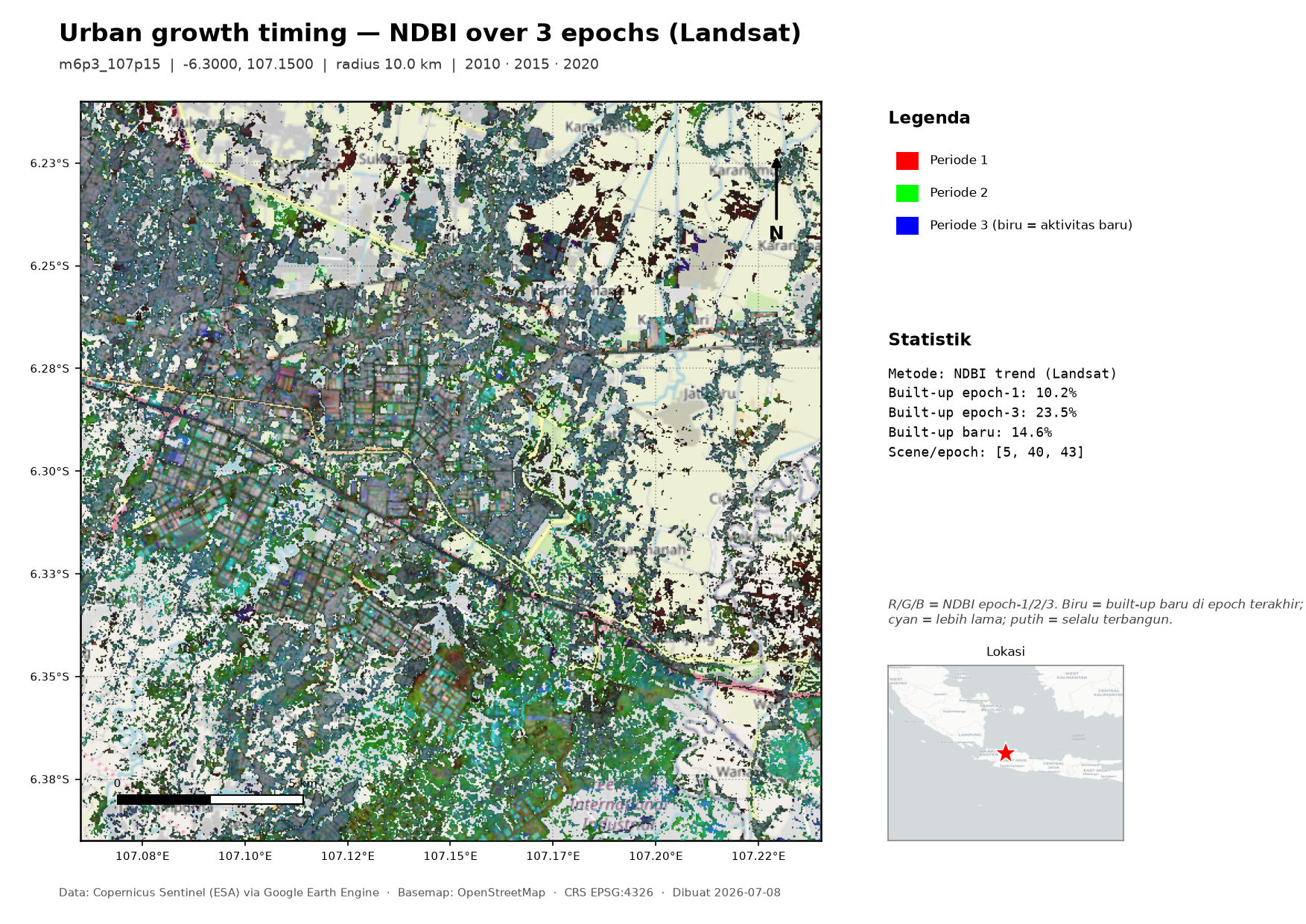
urban-trend over Cikarang/Bekasi (east Jakarta). Built-up grew 10% (2010) → 23% (2020), 15% newly built. White = built the whole time; blue/cyan = newer growth.urban-trend di Cikarang/Bekasi (timur Jakarta). Built-up tumbuh 10% (2010) → 23% (2020), 15% baru. Putih = terbangun terus; biru/cyan = pertumbuhan lebih baru.7 · Make a map productMembuat produk peta
Add --map to any run to render an A4-landscape map sheet (PDF + PNG) per product: OpenStreetMap basemap, the change layer, title, legend, a statistics panel, a location inset, coordinate grid, scale bar and north arrow.
Tambahkan --map pada run apa pun untuk membuat lembar peta A4 landscape (PDF + PNG) per produk: basemap OpenStreetMap, layer perubahan, judul, legenda, panel statistik, inset lokasi, grid koordinat, skala, dan panah utara.
earthchange -s mining --lat -3.333 --lon 122.25 --map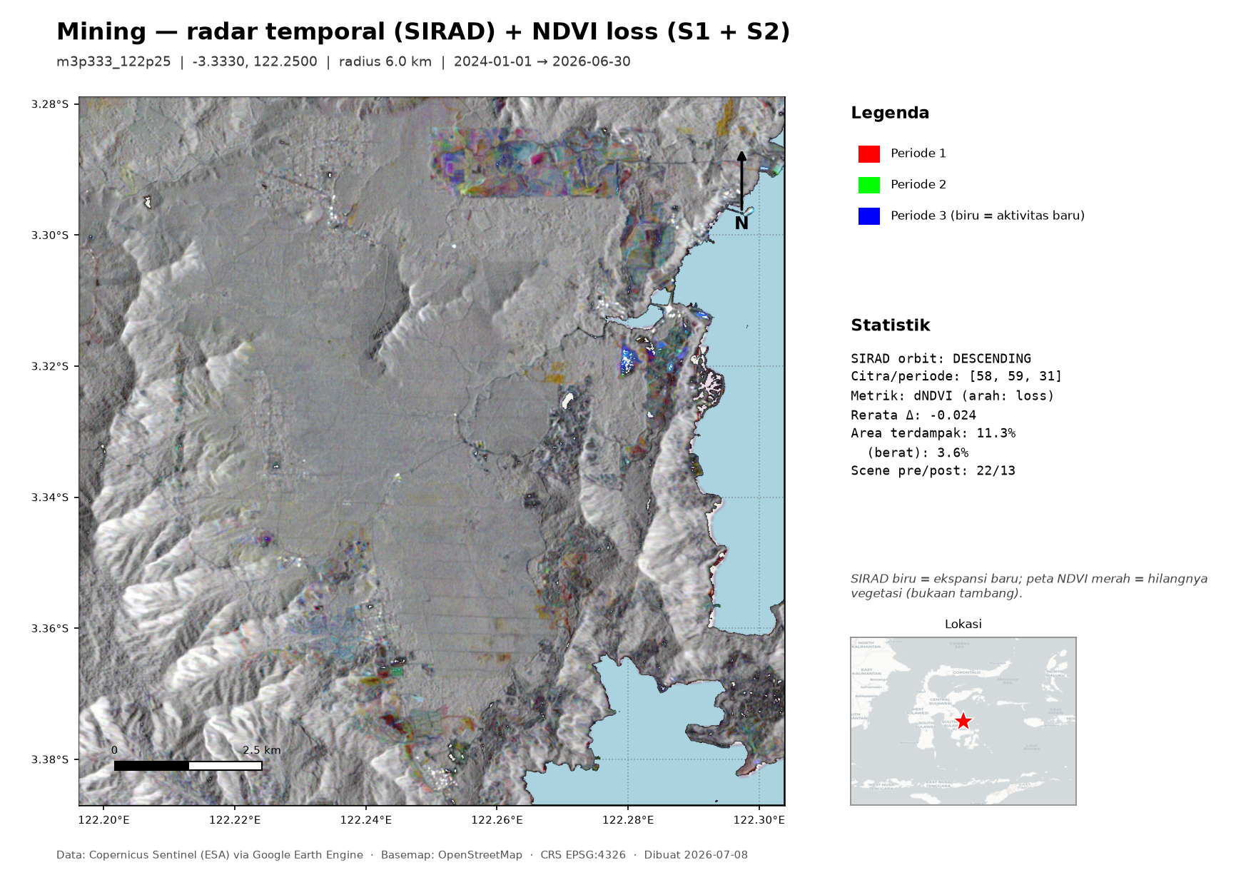
Already have results and just want to re-render (no Earth Engine needed)? Every run drops a .meta.json sidecar, so:
Sudah punya hasil dan ingin render ulang (tanpa Earth Engine)? Tiap run menulis sidecar .meta.json, jadi:
earthmap output/20260708-2226_deforestation_x_fac24e   # a run folder
earthmap output/<run>/mining_sirad_x.tif --basemap gray  # or one .tif
Maps land in maps/. Tweak the layout in mapmaker.py and re-run instantly.
Peta tersimpan di maps/. Ubah tata letak di mapmaker.py lalu jalankan ulang seketika.
8 · Adapt it to your own areaMenyesuaikan untuk area Anda
Pick a locationPilih lokasi
Find coordinates by right-clicking a spot in Google Maps (it copies lat, lon), or from OpenStreetMap. Choose a --radius to match the feature: a few km for a single mine or town, 10–20 km for a flood plain or a fire.
Cari koordinat dengan klik kanan di Google Maps (menyalin lat, lon), atau dari OpenStreetMap. Pilih --radius sesuai objek: beberapa km untuk satu tambang atau kota, 10–20 km untuk dataran banjir atau kebakaran.
Save a named presetSimpan preset bernama
Add reusable places to sites.py and call them with --site:
Tambahkan lokasi yang sering dipakai ke sites.py dan panggil dengan --site:
SITES = {
  "my_area": {
    "label": "My study area",
    "lat": 1.234, "lon": 103.456, "radius_km": 8.0,
    "sentinel2_date": "2026-06-15",
    "sirad_periods": [("2024-01-01","2024-12-31"),
                      ("2025-01-01","2025-12-31"),
                      ("2026-01-01","2026-06-30")],
    "ndvi_pre":  ("2023-01-01","2023-12-31"),
    "ndvi_post": ("2026-01-01","2026-06-30"),
  },
}
earthchange -s deforestation --site my_area --mapAdd a brand-new scenarioTambah skenario baru
Most scenarios are one dictionary entry in scenarios.py. To add, say, a moisture-change scenario using NDWI on a custom threshold you only add a registry entry — the generic optical-change engine does the rest:
Kebanyakan skenario hanya satu entri dictionary di scenarios.py. Untuk menambah, misalnya, skenario perubahan kelembapan memakai NDWI dengan ambang khusus, cukup tambahkan satu entri — mesin perubahan optik generik menangani sisanya:
"moisture": {
    "label": "Moisture change (NDWI)",
    "run": _optical("NDWI", "gain", 0.08, 0.20),  # index, direction, thresholds
    "radius": 10.0, "needs": "pre_post",
    "pre":  ("2023-01-01","2023-12-31"),
    "post": ("2025-01-01","2025-12-31"),
    "interpretation": "Greener = wetter.",
},
New spectral indices go in indices.py (a one-line normalised difference). Radar or bespoke methods get a small run_* function in scenarios.py.
Indeks spektral baru masuk ke indices.py (satu baris normalized difference). Metode radar atau khusus memakai fungsi run_* kecil di scenarios.py.
9 · Reproducibility & dataReproduksibilitas & data
- Data: Copernicus Sentinel-1 (radar) and Sentinel-2 (optical), free and open, courtesy ESA, processed in Google Earth Engine.
- AOI: a square centred on your coordinate (half-side = radius), axis-aligned in EPSG:4326.
- Orbit auto-selection: radar scenarios check both ascending and descending orbits and use whichever has imagery in every period.
- Outputs are regenerable, so results and maps are git-ignored; only code and this tutorial are versioned.
- Data: Copernicus Sentinel-1 (radar) dan Sentinel-2 (optik), gratis dan terbuka, dari ESA, diproses di Google Earth Engine.
- AOI: persegi berpusat di koordinat Anda (setengah-sisi = radius), sejajar sumbu di EPSG:4326.
- Pemilihan orbit otomatis: skenario radar memeriksa orbit ascending dan descending lalu memakai yang punya citra di tiap periode.
- Keluaran bisa dibuat ulang, jadi hasil dan peta di-git-ignore; hanya kode dan tutorial ini yang diversikan.
10 · TroubleshootingPemecahan masalah
| SymptomGejala | FixSolusi |
|---|---|
No Sentinel-2 scenes in pre/post window | Widen your --pre/--post dates or increase --radius. Very cloudy tropics may need a longer window.Perlebar tanggal --pre/--post atau perbesar --radius. Tropis sangat berawan mungkin butuh jendela lebih panjang. |
No orbit covers all periods | Enlarge the radius or shift the period dates; Sentinel-1 coverage is sparse in some years/areas.Perbesar radius atau geser tanggal periode; cakupan Sentinel-1 jarang di sebagian tahun/area. |
| Earth Engine auth errorsGalat autentikasi Earth Engine | Usually a wrong working directory: the key at scripts/config/ee-geodetic.json is only found when you run from the repo root. Pass --ee-key /path/to/ee-geodetic.json, set EARTHCHANGE_EE_KEY, copy the key to ~/.config/earthengine/ee-geodetic.json, or re-run earthengine authenticate.Biasanya direktori kerja salah: kunci di scripts/config/ee-geodetic.json hanya ditemukan saat dijalankan dari root repo. Berikan --ee-key /path/ke/ee-geodetic.json, set EARTHCHANGE_EE_KEY, salin kunci ke ~/.config/earthengine/ee-geodetic.json, atau jalankan ulang earthengine authenticate. |
Basemap missing / Basemap hilang / EPSG code unknown | A stale external PROJ database (e.g. from an OTB install) is shadowing PROJ. The tool clears PROJ_LIB; if it persists, unset PROJ_LIB.Basis data PROJ eksternal usang (mis. dari OTB) menutupi PROJ. Alat menghapus PROJ_LIB; bila masih, jalankan unset PROJ_LIB. |
| Direct GeoTIFF download refusedUnduhan GeoTIFF langsung ditolak | Very large AOIs exceed Earth Engine's limit — reduce --radius, or use --drive to export to Google Drive.AOI sangat besar melewati batas Earth Engine — kecilkan --radius, atau pakai --drive untuk ekspor ke Google Drive. |
11 · Further readingBacaan lanjut
- Zha, Gao & Ni (2003). Use of NDBI in automatically mapping urban areas from TM imagery. Int. J. Remote Sensing 24(3).
- Key & Benson (2006). Landscape Assessment: the Normalized Burn Ratio (NBR/dNBR). USDA Forest Service, FIREMON.
- UN-SPIDER. Recommended Practice: Flood Mapping with Sentinel-1 SAR in Google Earth Engine.
- UN-SPIDER. Normalized Burn Ratio — in detail.
- Earth Lab. Work with the Differenced Normalized Burn Index (dNBR).
- Google Earth Engine. Sentinel-1 SAR guide · Sentinel-2 SR Harmonized.