Irrigation performance

SI, CU, RI per tertiary block for a Daerah Irigasi

The idea

The final step turns the satellite maps into operational irrigation indicators for a Daerah Irigasi (DI), computed per tertiary block (petak tersier). Three standard indices (FAO / Bos 1985) summarise how well the network delivers water:

Index	Meaning	Question it answers
SI — Satisfaction Index	adequacy	Is each block getting enough water?
CU — Christiansen Uniformity	uniformity	Is water spread evenly across the DI?
RI — Reliability Index	dependability	Does each block stay adequate over time?

We demonstrate on DI Klambu (Grobogan, Central Java; 653 tertiary blocks), whose block boundaries and reference results ship with the repository.

What this chapter demonstrates vs the full method

To stay laptop-runnable, the steps below build the water balance from Sentinel-1 (crop coefficient / Kc) plus CHIRPS rainfall and reference ET. The full operational method also fuses Sentinel-2 and Landsat optical imagery to estimate ET / Kc more accurately — that multi-sensor fusion is the production upgrade, kept out of this hands-on chapter so it remains reproducible on a laptop.

Step 1 — Crop water demand: the Kc map

Growth phase → crop coefficient (Kc) links what the satellite sees to how much water the crop needs. produce_kc_map.py estimates days-after-transplant from the VH flooding trough and maps it onto the FAO-56 rice 110-day curve (Kc 1.05 → 1.20 → 0.95 → 0).

Pass your VH stack and paddy mask with --stack / --paddy-mask. --period-band is the band index to target (it uses that band plus the 9 before it, so it needs ≥10 bands of history — with the 18-band sample, use 10–18):

python produce_kc_map.py --period-band 14 --out kc_sample \
    --stack data/sample/klambu_vh_2024.tif \
    --paddy-mask consensus_sample/consensus_paddy_map.tif
# → kc_sample/kc_band14.tif  (Kc per active-paddy pixel)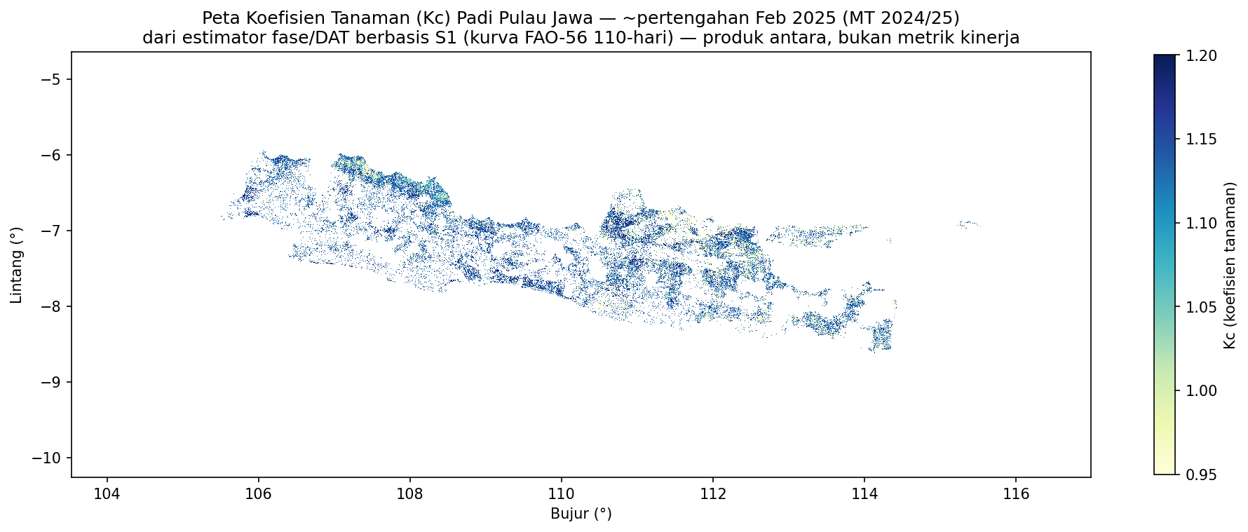

Crop-coefficient (Kc) map, MT 2024/25 — the bridge from phenology to water demand.

Expect a sparse result on the toy AOI

Because the sample paddy mask is small (and built from just a few periods), the Kc map — and the indices downstream — may cover very few pixels. The steps below demonstrate the mechanics, not a representative result; use a fuller multi-year stack and more periods for meaningful output.

Step 2 — Water balance (rainfall vs demand)

The Satisfaction Index compares supply (rainfall — and, where available, gate/staff-gauge flows) against demand (Kc × reference evapotranspiration). The project uses CHIRPS rainfall and ET; the shipped daily series for Klambu live in 2026/irrigation_performance/ and 2026/irrigation_performance_2024_s1kc/.

Satellite-only vs water-referenced SI

Without gate-sensor data, SI is computed from active-paddy detection (a satellite proxy for adequacy). Referencing SI to actual water (gate openings) is the field-validation step planned for a later campaign — see the reports. Be explicit about which you report.

Step 3 — Compute SI / CU / RI per block

calculate_irrigation_indices.py ties it together — it reads your per-period paddy predictions and the tertiary-block boundaries (klambu.gpkg, block-id field norec), zonally aggregates the active- paddy signal, and writes the three indices per block.

python calculate_irrigation_indices.py \
    --predictions-dir predictions_sample/2024 \
    --periods 13 15 17 19 21 23 \
    --di-boundary 2026/irrigation_performance/klambu.gpkg \
    --output-dir irrigation_results/klambu_2024 \
    --confidence-threshold 0.7

Outputs include per-block index CSVs, a DI-level summary, and time-series/histogram quick-looks in irrigation_results/klambu_2024/.

The repository already ships reference results you can inspect immediately:

head 2026/irrigation_performance/reliability_block_results.csv
cat 2026/irrigation_performance/performance_summary.txt

Step 4 — Map the indices per block

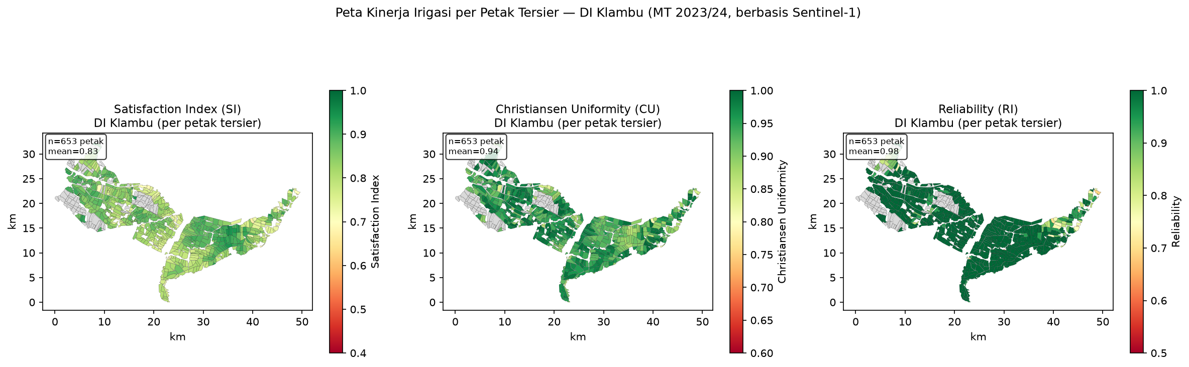
make_irrigation_maps.py renders the three choropleth panels. It reads the per-block CSVs from ./results_csv/ (a fixed location) and joins them to klambu.gpkg. The quickest way to see it is with the shipped reference results:

mkdir -p results_csv
cp 2026/irrigation_performance/uniformity_block_results.csv results_csv/
cp 2026/irrigation_performance/reliability_block_results.csv results_csv/
python make_irrigation_maps.py
# → writes 2026/figures/fig_irrigation_klambu_maps.png

(To map your run instead, copy the CSVs produced in Step 3 into results_csv/ before running.)

Per-tertiary-block irrigation indices for DI Klambu (SI, CU, RI).

Reading the result

For DI Klambu the full study finds:

Index	Value	Category (FAO/Bos 1985)
SI	0.83	Very good
CU	0.93	Very good
RI	0.98	Very good

But the operationally useful output is the spatial diagnostic: the system flags 10 problematic blocks (RI < 0.75), 7 of them at the tail-end of the tertiary network — the classic head–tail inequity. Instead of inspecting all 653 blocks, the BBWS can target those 10 — the core value proposition of a satellite approach.

Suggested performance thresholds (P3A contracts)

A tiered scheme lets adoption start conservative and tighten over time. Tier 1: SI ≥ 0.75, CU ≥ 0.80, RI ≥ 0.70, plus cropping index ≥ 1.5.

Where to go next

You have reproduced the full chain on a sample DI. To scale up you would: process more Sentinel-1 periods and years, extend to more DIs, and — the key upgrade — add field validation to water-reference SI and calibrate the phase algorithm.

For the more accurate growth-phase product that underpins Kc, continue to Going further: S1+S2 fusion.