Planting index
Counting cropping cycles: 1×, 2×, 3× per year
🌐 English · Bahasa Indonesia →
The idea
The planting index (cropping intensity, indeks pertanaman) answers how many times a field is planted in one agricultural year. We derive it directly from the VH time series with a data-driven cycle counter: no fixed calendar, no absolute-dB threshold.
Each rice cycle is a flood trough → canopy peak swing. A per-pixel state machine walks the time series and counts a cycle whenever VH rises by at least a minimum amplitude (≈4 dB) above a running minimum, then re-arms after it falls back down. The number of complete cycles is the planting index for that pixel (reported 1 / 2 / 3+).
Counting periods a pixel “looks like paddy” over-counts (transient look-alikes inflate it). Requiring a full flood→canopy amplitude swing is physically grounded and rejects those artefacts.
Step 1 — Validate the counter (optional)
cropping_intensity.py can sanity-check its vectorized counter against an independent rice map (single/double/triple classes) before running on your stack:
python cropping_intensity.py --mode validate \
    --stack data/sample/klambu_vh_2024.tif        # or your own multi-year stack
The mean detected cycles should increase monotonically from the single- to the triple-crop reference class — evidence the counter tracks real intensity. Verified output on the full Java stack:
Open-SEA CI=1: n=400 mean detected=1.77
Open-SEA CI=2: n=400 mean detected=2.06
Open-SEA CI=3: n=400 mean detected=2.31
Step 2 — Compute cropping intensity on the AOI
Run the full mode on your AOI stack. The candidate mask makes the result rice-specific — use your paddy consensus (recommended) or a baku-sawah/cadastre layer; without one, use --no-candidate (cycles only, less specific).
python cropping_intensity.py --mode full \
    --stack <your-multi-year-vh-stack.tif> \
    --candidate-mask consensus_sample/consensus_paddy_map.tif \
--output cropping_intensity_sample--mode full counts cycles over the MT 2024/25 agricultural-year window, which the script reads from bands 25–56 of the combined 2024–2026 stack. The small single-year sample AOI (18 bands) does not cover that window — point --stack at your full multi-year stack, or edit MT_BANDS in the script for a different band range. The --mode validate step above does run on the sample.
On the small single-year sample, the within-year consensus mask (few periods, strict thresholds) can be nearly empty, so the cropping-intensity map here is sparse and illustrative only — it shows the mechanics, not a representative product. For a meaningful map, use more periods and the full multi-year stack.
Outputs:
cropping_intensity_sample/
├── cropping_intensity.tif   # uint8: 0 non-paddy, 1 / 2 / 3(=3+) crops
├── paddy_mask.tif           # 1 where ≥1 cycle
└── statistics.txt           # area per class + aggregate index
statistics.txt reports the aggregate cropping index (mean cycles over paddy) and the ha in each class.
- Anomalous ~0 dB bands (acquisition/processing gaps) are auto-detected and interpolated — two such bands otherwise fake an extra canopy swing and inflate the index.
- Pixel area at 50 m ≈ 0.25 ha; the script uses this, so areas are correct.
What the full study shows
On Java for MT 2024/25, the aggregate index is ≈1.62 on the stable-consensus footprint, with a clear spatial pattern — triple-cropping concentrates along water-secure corridors (Pantura, Bengawan Solo).
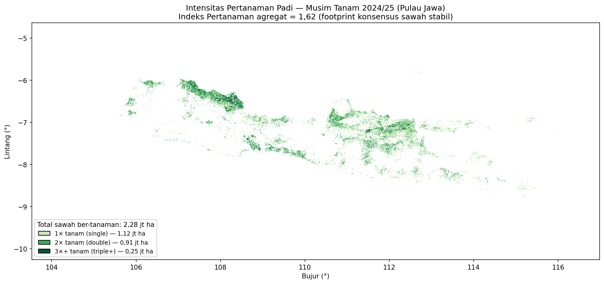
An inter-annual comparison on identical pixels rose from IP 1.45 (MT 2023/24) → 1.63 (MT 2024/25) — the planted area barely changed, but intensity went up (more double- and triple-cropping), consistent with post-El-Niño water recovery. That signal — climate variability driving cropping intensity — is the scientifically interesting part of the multi-year record.
Choosing the footprint
The cropping-intensity extent depends on the candidate mask you pass:
- your consensus mask → the map nests inside your paddy map (recommended, coherent);
- a cadastre/baku-sawah mask → the map is clipped to the official footprint;
--no-candidate→ cycles over all land (rejects nothing non-rice — use with care).
Keep the footprint consistent with the paddy map so the two products tell one story.
Next: convert phenology into water demand and compute irrigation performance → Irrigation performance.